Article
Nonlinear Model Predictive Control Using Robust Fixed Point Transformation-Based Phenomena for Controlling Tumor Growth
Bence Czakó *,†and Levente Kovács *,†ID
Physiological Controls Research Center, EKIK, Obuda University, 1034 Budapest, Hungary
* Correspondence: czako.bence@stud.uni-obuda.hu (B.C.); kovacs.levente@nik.uni-obuda.hu (L.K.)
† These authors contributed equally to this work.
Received: 31 August 2018; Accepted: 17 October 2018; Published: 25 October 2018 Abstract: In this paper a novel control strategy is introduced in order to create optimal dosage profiles for individualized cancer treatment. This approach uses Nonlinear Model Predictive Control to construct optimal dosage protocols in conjunction with Robust Fixed Point Transformations which hinders the negative effect of inherent model uncertainties and measurement disturbances.
The results are validated by extensive simulation on the proposed control algorithm from which conclusions were drawn.
Keywords: physiological control; nonlinear systems; model predictive control; robust fixed point transformation
1. Introduction
In the past decades, physiological systems gained attention among control engineers.
This particular interest covers a significant variety of topics including automated anesthesia [1], diabetes control [2] and hormonal regulation [3]. Tumor growth control is no exception as cancerous diseases are responsible for 1,359,500 deaths in the European Union annually, based on [4]. Because of the physiological complexity of tumor growth, the topic has been intact for decades. However in the end of the 20th century, progress in cancer research delivered mathematical models that are able to encapsulate the underlying mechanisms. An important result was Targeted Molecular Therapies (TMTs) which exploit certain cancer specific processes that corresponds to the vascluar growth of tumors, thus hampering its effect in the body of the patient. This approach led to the famous Hahnfeldt model, which was introduced by [5], and has been used thoroughly since its development among control engineers.
The primary issue with TMTs is that the developed drugs are exceedingly expensive, thus availability for the vast majority is limited. A possible solution to this issue is to apply optimal control techniques to the existing tumor growth model that incorporates the expenses of the drug while maintaining a reasonable treatment plan i.e., minimizing the costs and the treatment time.
Several algorithms were proposed in the literature based on linear design methods [6] and nonlinear techniques [7]. Many evidence [8,9] and practical consideration, such as unstable behaviour of the linearised system and significant discrepancies in terms of model parameters between different patients, suggest that nonlinear methods have to be employed. In spite of these facts, a novel approach is presented in this paper, which combines the optimal behaviour of the Nonlinear Model Predictive Control (NMPC) in conjunction with the error insensitive traits of the Robust Fixed Point Transformation (RFPT) based nonlinear adaptive control. In a previous work, the NMPC architecture was deployed in order to tackle the optimization issue [10]. However as it was indicated
Machines2018,6, 49; doi:10.3390/machines6040049 www.mdpi.com/journal/machines
in [11], the states of the system are not measurable due to large parameter uncertainties and model imperfections; therefore, an adaptive approach is suggested. The problem with the RFPT approach is that it can not guarantee an optimal dosing protocol by itself. While it is locally robust, it can not track constant references which are far from the initial value. In spite of these facts, a combined approach is presented here, which may also be applicable for other physiological systems as well that has significant parameter variations in the nominal model.
The paper first introduces the underlying model of the system and the important theoretical background of both the NMPC and the RFPT method. After the introduction, the connection is presented between the two methods with a detailed explanation of the problems that has to be solved from a control engineering aspect. In the end of the paper, numerical simulations are presented in order to verify the behaviour of the controller, on which conclusions are drawn.
2. System Model
Since anti-angiogenic therapy has emerged, many approaches have been considered by various authors. A comprehensive study on tumor growth models can be found in [12] from a control engineering point of view. However, advancements in cancer research have carried out new results, which indicate that the currently existing models do not incorporate important alternate vascularization methods, as pointed out in [13]. In order to overcome these issues, different models were developed by [14,15] that describes the growth process accurately, which was validated by mice experiments.
However, in this article, the famous Hahnfeldt model [5] is used, which does not cover every physiological aspect, but rather facilitates the comparison between the presented control algorithm and previously employed approaches.
Based on the work of [6], many simplifications can be attained on the original Hahnfeldt model, such as elimination of terms that are shown to be negligible by experiments [5], or merging variables that tend to move together [16]. The modified equations of motion can be described as:
x˙1=−λx1lnx1 x2
˙
x2=bx1−dx2/31 x2−ex2g(t),
(1)
wherex1denotes the tumor volume (mm3), which is the output of the system,x2is the volume of the tumor vasculature (mm3),λis the growth parameter of the tumor (1/day),bis the angiogenic factor (1/day),ddescribes the cellular blocking mechanisms of the vasculature (1/day·mm2),eis the inhibition of the vasculature by the drug (kg/day·mg), andg(t)is the concentration of the administered inhibitor (mg/kg). The parameters were chosen according to [17], which are presented in Table1.
Table 1.Simulation parameters.
λ b d e
0.192 5.85 0.00873 0.66
It is worth mentioning that the underlying system model describes a positive dynamical system, which entails that the control signal must remain positive for all times. Previous simulations showed that when the input signal is zero, the model attains a steady state ofx1=x2= 1.734×10⁴(mm3). This steady state yields a worst case scenario, so that the controller is designed according to this initial value in order to deal with minor initial tumor volumes as well. Because anti-angiogenic therapy does not eradicate the tumor completely, the objective is to shrink the volume to such an extent that it does not jeopardise the health of the patient. The model contains a major singularity atx1=x2= 0 (mm3) that corresponds to the previously indicated behaviour of the therapy, which implies that the control objective can not be zero value. In particular the tumor is said to be in safe steady state if its volume
does not exceed 10 (mm3); hence from the controllers perspective it is sufficient to bring the tumor volume in this region.
3. Control Algorithm
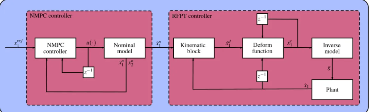
In this section, the combined NMPC-RFPT approach is introduced with the necessary design steps for the simplified Hahnfeldt model as a primary example. The idea shares similar traits of the robust NMPC approach that can be seen in [18]; however, the second optimization loop is replaced by the RFPT controller. This decreases the computational burden of the dual NMPC solution and makes the design steps easier, as it does not require to construct terminal cost and sets to ensure a robust operation of the controller. This technique also overcome several obstacles concerning the RFPT method. The NMPC block provides an optimal trajectory for set point tracking, as an output of the nominal model, that can be used by the RFPT controller. This solves the set point tracking problem of the RFPT controller by providing an appropriate nominal trajectory prescription, in conjunction with the non-optimal behaviour of the RFPT technique. If the plant and the nominal model has the same parameter values, the RFPT controller can be tuned to produce minor tracking error, thus the plant trajectory does not deviate significantly from the nominal, which entails that the output isessentiallyoptimal. If uncertainties are present in the plant, then the RFPT controller tries to reduce these deviations which renders the control loop robust. It should be also noted that the nominal trajectory, which is provided by the NMPC block, can be computed offline which makes the method computationally attractive. This means in practice that instead of solving a complex nonlinear optimization in each control cycle, one step of iteration (7) has to be computed which is faster.
3.1. The Nonlinear Model Predictive Controller
The NMPC consists of three main ingredients, namely, prediction, optimization, and execution.
The controller uses the plant measurement in order to predict the behaviour of the system based on the discrete model, which is then used in a cost function. This essentially means the construction of a complicated cost function that has to be minimized by the input sequence for each prediction step, which implies the use of nonlinear optimization solvers. From the optimal control sequence, the first element is applied to the plant and the cycle repeats. The operation of the controller can be summarized in the Optimal Control Problem (OCPNn), based on [19] as:
arg min
u(·)∈UN(x0)
JN(n,x0,u(·)):=
N−1 k=0
∑
`(n+k,xu(k,x0),u(k)) s. t.xu(0,x0) =x0, xu(k+1,x0) = f(xu(k,x0),u(k)),
(2)
where x0 = x(n)is the measurement of states in the nth control cycle, N denotes the length of the optimization horizon, the valueu(·) ∈UN(x0)represents a vector of predicted input values of dimensionNfrom the feasible setUN, function`(n+k,xu(k,x0),u(k))is the cost function,JNis the total cost function that has to be minimized, andxu(k+1,x0) = f(xu(k,x0),u(k))is responsible for the prediction stage with initial conditionxu(0,x0) =x0. Note that the prediction equation describes a discrete time system in the form ofx+ = f(x,u). This implies in particular that the continuous time system must be discretized, therefore the system model takes the form of:
x+1 =x1+∆t[−λ1x1ln(x1/x2)]
x+2 =x2+∆t[bx1−dx12/3x2−ex2g] (3) in which∆tis the time step of the discretization. In (2), the left side of the prediction corresponds to the state variables in (3), namelyxu(k+1,x0) = [x+1 x+2]T, and the function f(xu(k,x0),u(k))is the vector valued function on the right-hand side of the discretization equation. It is worth mentioning
that different discretization methods can be employed which could lead to more accurate results, thus improving the overall robustness of the NMPC controller in exchange for computational effort.
According to [19], the cost function can be defined as
`(k,x1,u) =ζ
x1−xre f(k)2+ξ
u−ure f(k)2 (4) whereζandξare control parameters,x1is the tumor volume,xre f(k)is the time-varying reference signal with ure f(k) as the desired input signal at prediction time k, and k·k is the Euclidean norm. Equation (4) allows the use of time varying references; however, in this case a constant reference is proposed, soxre f(k)∈ [1; 10](because of the singularity in the model atx1 = x2 =0), andure f(k) =0, ∀k∈N. For technical reasons, in every control cycle, the calculated predicted values u(·)is used in the next step by the nonlinear optimization algorithm as an initial guess.
3.2. The Robust Fixed Point Transformations Based Controller
The RFPT method is a novel nonlinear control technique which was introduced by [20] and proven to be effective in many control problems providing accurate results. Its operation can be described with the realized-response scheme. Theoretically, if one calculates the input signal for an arbitrary trajectory by inverting the dynamics of the model, then it is possible to steer the system along this trajectory by applying the calculated input signal to the plant, if there are no uncertainties between the nominal and physical systems (this will be called the desired response). However, in the vast majority of cases this is not true due to modelling imperfections, or parameter variations. This causes a realized response which differs significantly from the desired one, thus the control objective can not be achieved. The RFPT method solves this issue by deforming the desired input trajectory, so that the calculated input signal produces the desired response of the plant. A more elaborate description can be found in [20–22].
The method first uses a kinematic part which can be completely determined by the order of the system, that is the highest derivative of the states in the system model. The kinematic equation is given by:
eint(t) = Z t
t0(qn(τ)−q(τ))dτ , (d
dt+Λ)n+1eint=0
(5)
whereqnis the reference trajectory,qis the measured state,nis the order of the system, andΛis a control parameter. Since the highest derivative isn=1 and the controlled variable isx1, the expression takes the form of:
eint(t) = Z t
t0(x1n(τ)−x1(τ))dτ ,
˙
xd1=Λ2eint+2Λe+x˙1n.
(6)
In (6),xn1denotes the reference tumor volume that is a decreasing function with respect to time.
In the combined approach this will be the output of the nominal system model of the NMPC part.
After the kinematic part, the output ˙xd1is used by the deform function which is defined as:
G(r|rd)de f= (r+K)[1+Btanh(A[f(r)−rd])]−K G(rd∗|rd) =rd∗, if f(rd∗) =rd
G(−K|rd) =−K, ifr=−K
(7)
whence the iteration is achieved byrn+1 = G rn|rd
. In (7), f(r)is the measured signal,rd is the output of the kinematic block that is ˙xd1,r∗dis the solution of the fixed point problem for which the realized response of the system coincides with the desired trajectory, and A,B,Kare free control
parameters. Using the deformed trajectory, the output can be calculated from the inverse model, which now has to be expressed. Taking the first equation from (1) and rearranging the terms leads to:
x2=x1exp
−λxx˙1
1
−1
. (8)
Differentiation of the previous equation yields:
˙ x2=
x˙1exp
− x˙1 λx1
+x1exp
− x˙1 λx1
x˙1x1λ−λx˙21 (λx1)2
exp
− x˙1 λx1
2 (9)
from which the following form can be obtained by simplification:
˙
x2= λx˙1x1+x¨1x1−x˙21
fλx1 (10)
In the simplified equationf denotes the exponential term in (9). This equation can be substituted into the second equation in the system model (1), together with Equation (8). By rearranging the terms, g(t)can be expressed as:
g(t) =−λx˙1x1+x¨1x1−x˙21+λdx8/31 −λbx1f
λex21 (11)
which is the inverse model of the system. Applying the output of the deform function to the inverse model leads to a proper control signalg(t), which drives the system along the desired trajectory.
3.3. The Combined Approach
The last step in the design process is to determine the parameters of the controllers. A possible path is to tune the NMPC controller separately to the nominal plant by adjusting the values ofξandζ, so that it meets the design criterion, or using other more sophisticated techniques from the NMPC literature. If the NMPC controller is tuned, the output of the nominal system can be used as an input of the RFPT controller so that parametersA,KandBcan be determined by numerical simulations on the nominal plant. Because of its novelty, the RFPT method has no exact tuning techniques yet.
However, several thumb rules exist which alleviate the tuning process;Bis either 1 or−1,Kis usually a big number with the magnitude of 105, andA=1/(10·K). A schematic depiction of the controller architecture can be seen in Figure1.
Version October 9, 2018 submitted toMachines 5 of 9
˙ x2=
˙ x1exp
(
− x˙1 λx1
) +x1exp
(
− x˙1 λx1
) (x˙1x1λ−λx˙21 (λx1)2
)
exp (
− x˙1 λx1
)2 (9)
from which the following form can be obtained by simplification:
139
˙
x2=λx˙1x1+x¨1x1−x˙21
fλx1 (10)
In the simplified equationfdenotes the exponential term in (9). This equation can be substituted into the second
140
equation in the system model (1), together with equation (8). By rearranging the terms,g(t)can be expressed
141
as:
142
g(t) =−λx˙1x1+x¨1x1−x˙21+λdx8/31 −λbx1f
λex21 (11)
which is the inverse model of the system. Applying the output of the deform function to the inverse model leads
143
to a proper control signalg(t), which drives the system along the desired trajectory.
144
3.3. The combined approach
145
The last step in the design process is to determine the parameters of the controllers. A possible path is to
146
tune the NMPC controller separately to the nominal plant by adjusting the values ofξ andζ, so that it meets
147
the design criterion, or using other more sophisticated techniques from the NMPC literature. If the NMPC
148
controller is tuned, the output of the nominal system can be used as an input of the RFPT controller so that
149
parametersA,KandBcan be determined by numerical simulations on the nominal plant. Because of its novelty,
150
the RFPT method has no exact tuning techniques yet. However, several thumb rules exist which alleviates the
151
tuning process;Bis either 1 or−1,Kis usually a big number with the magnitude of 105, andA=1/(10·K).
152
A schematic depiction of the controller architecture can be seen on Fig.1.
153
controllerNMPC
z−1
Nominal
model Kinematic
block Deform
function Inverse
model
Plant z−1
z−1
xre f1 u(·) x˙n1 x˙d1
˙ x1
g
˙ xr1
NMPC controller RFPT controller
xn1 xn2
Figure 1.Schematic depiction of the combined NMPC-RFPT approach 4. Simulation results
154
Multiple simulations were conducted in order to ensure the appropriate operation of the controller.
155
In order to mimic real behaviour, the NMPC controller operates on the plant once every day with zero
156
order hold. The prediction time step was 1/24(day)with a horizon ofN=24·14=336, which predicts
157
the evolution of the system for two weeks. Control parameters ζ =100, ξ =1 produced acceptable
158
results in terms of tumor volume reduction and total inhibitor concentration, with a maximum input signal
159
restriction of 25 (mg/kg). For this nominal trajectory, the parameters of the RFPT controller was set as
160
K=5.3·1010,A=1/(1011), B=−1, by empirical tuning, which produced sufficiently small tracking errors.
161
Figure 1.Schematic depiction of the combined NMPC-RFPT approach.
4. Simulation Results
Multiple simulations were conducted in order to ensure the appropriate operation of the controller.
In order to mimic real behaviour, the NMPC controller operates on the plant once every day with zero order hold. The prediction time step was 1/24 (day) with a horizon ofN= 24×14 = 336, which predicts the evolution of the system for two weeks. Control parametersζ=100, ξ=1 produced acceptable results in terms of tumor volume reduction and total inhibitor concentration, with a maximum input signal restriction of 25 (mg/kg). For this nominal trajectory, the parameters of the RFPT controller was set asK= 5.3×10¹⁰,A= 1/(1011),B=−1, by empirical tuning, which produced sufficiently small tracking errors. The simulation step was∆t=10−3(day), with time intervalt∈[0; 100].
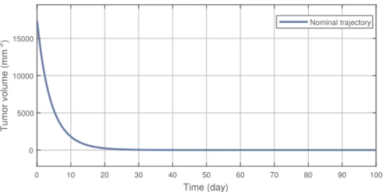
On Figure2the nominal trajectory is presented which was created by the NMPC controller.
After the 100th day the tumor volume was 1.083 (mm3), which is close to the desired setpoint value of x1= 1 (mm3). This result can be improved by increasing the prediction horizon; however, it affects the computational time significantly, thus it was not applied here. The tumor reduces under 10 (mm3) volume in 31 (days), with an inhibitor concentration of 765.7 (mg/kg). Compared to the results in [10]
this is clearly an improve in terms of concentration during the transient phase, i.e., the amount of medication given to the patient until the tumor volume reaches 10 (mm3).
0 10 20 30 40 50 60 70 80 90 100
Time (day) 0
5000 10000 15000
Tumor volume (mm3)
Nominal trajectory
Figure 2.The nominal trajectory produced by the NMPC controller.
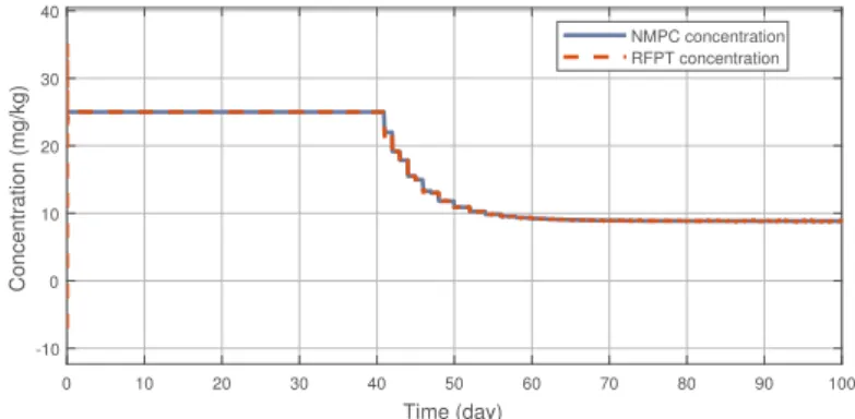
Figure3illustrates the tracking error of the RFPT controller on the nominal trajectory. It can be seen that the error decreases to zero almost in ten days while its values in the transient phase does not exceed 15 (mm3), which can be considered negligible. The difference between the two control signal can be scrutinised on Figure4. It can be seen that the RFPT input signal matches its NMPC counterpart almost everywhere, thus it does not violate the bounds on the control input. It should be noted, however, that there is a jump at the beginning of the control cycle which can be attributed to numerical imprecisions. The reduction of tumor and vasculature volume can be seen on Figure5.
0 10 20 30 40 50 60 70 80 90 100
Time (day) -15
-10 -5 0 5
Tumor volume error (mm3) Tracking error
Figure 3.Tracking error of the RFPT controller.
0 10 20 30 40 50 60 70 80 90 100 Time (day)
-10 0 10 20 30 40
Concentration (mg/kg)
NMPC concentration RFPT concentration
Figure 4.Administration protocols of the RFPT and the NMPC controller.
0 10 20 30 40 50 60 70 80 90 100
Time (day) 0
5000 10000 15000
Volume (mm3)
Vasculature volume Tumor volume
Figure 5.The reduction of the tumor volume.
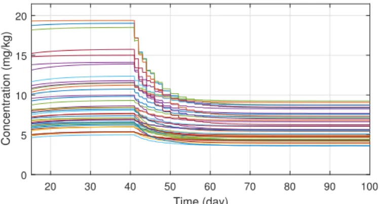
In order to ensure the robustness of the controller, different system parameter configurations were simulated. The parameters were chosen with Latin Hypercube Sampling from the interval[0; 1], which was then scaled to the order of magnitude for each parameter and added to their nominal values.
In total fifty different parameter configuration was tested, which revealed that the system is very sensitive for parameterd, but for the other three the controller is able to manage even extreme cases as well. On Figure6one can see the tracking errors which are caused by the parameter uncertainties between the nominal and real models. The maximal error has increased significantly, but the error vanishes in ten days and the maxima is negligible compared to the initial value of the tumor volume.
Simulations also revealed that the robustness can be increased by adjusting the value ofΛin the kinematic part; henceΛwas altered toΛ=0.5. On Figure7the different administration protocols are shown. It is worth noting that their shape resembles the nominal case in Figure4and also their values do not violate the 25 (mg/kg) constraint prescription.
0 2 4 6 8 10
Time (day) -60
-40 -20 0 20 40 60 80
Tumor volume error (mm3)
Figure 6.Tracking errors under parameter uncertainties.
20 30 40 50 60 70 80 90 100 Time (day)
0 5 10 15 20
Concentration (mg/kg)
Figure 7.Administration protocols under parameter uncertainties.
5. Conclusions
In this paper, a novel control method was introduced that uses the NMPC and RFPT methods in order to achieve robust optimal control of an anti-angiogenic tumor growth model. A design procedure was introduced, so that the approach can be used in different control problems that require a robust optimal control. Simulations showed that the proposed algorithm can tackle many issues posed by parameter uncertainties and modelling imperfections. The algorithm combined with previous results on discrete control with large sampling time of the Hahnfeldt model could result in a final solution to the individualized anti-angiogenic problem. Further research has to focus on auto tuning of the RFPT controller and also the possibility to include a feedback part for the NMPC part of the controller.
Author Contributions: Conceptualization, B.C. and L.K.; Data curation, B.C.; Formal analysis, B.C.; Funding acquisition, L.K.; Investigation, L.K.; Methodology, L.K.; Project administration, L.K.; Resources, L.K.; Software, B.C.; Supervision, L.K.; Validation, B.C.; Visualization, B.C.; Writing—original draft, B.C.; Writing—review &
editing, L.K.
Funding:This project has received funding from the European Research Council (ERC) under the European Union’s Horizon 2020 research and innovation programme (grant agreement No 679681). Bence Czakó was supported by the UNKP-17-2/I. New National Excellence Program of the Ministry of Human Capacities.
Conflicts of Interest:The authors declare no conflict of interest.
References
1. Ionescu, C.M.; Copot, D. Guided closed loop control of analgesia: Are we there yet? In Proceedings of the 2017 IEEE 21st International Conference on Intelligent Engineering Systems (INES), Larnaca, Cyprus, 20–23 October 2017; p. 137142.
2. Kovács, L. A robust fixed point transformation-based approach for type 1 diabetes control. Nonlinear Dyn.
2017,89, 2481–2493. [CrossRef]
3. Churilov, A.; Medvedev, A.; Shepeljavyi, A. Mathematical model of testosterone regulation by pulse- modulated feedback. In Proceedings of the 2007 IEEE International Conference on Control Applications, Singapore, 1–3 October 2007.
4. Malvezzi, M.; Carioli, G.; Bertuccio, P.; Rosso, T.; Boffetta, P.; Levi, F.; Vecchia, C.L.; Negri, E. European cancer mortality predictions for the year 2016 with focus on leukaemias. Ann. Oncol. 2016,27, 725–731.
[CrossRef] [PubMed]
5. Hanhfeldt, P.; Panigrahy, D.; Folkman, J.; Hlatky, L. Tumor development under angiogenic signaling:
A dynamical theory of tumor growth, treatment response, and postvascular dormancy. Cancer Res.1999, 59, 4770–4775.
6. Sapi, J.; Drexler, D.A.; Kovacs, L. Parameter optimization of H infinity controller designed for tumor growth in the light of physiological aspects. In Proceedings of the 2013 IEEE 14th International Symposium on Computational Intelligence and Informatics (CINTI), Budapest, Hungary, 19–21 November 2013.
7. Drexler, D.A.; Sápi, J.; Kovács, L. Positive nonlinear control of tumor growth using angiogenic inhibition.
IFAC-PapersOnLine2017,50, 15068–15073. [CrossRef]
8. Czako, B.G.; Kosi, K. Novel method for quadcopter controlling using nonlinear adaptive control based on robust fixed point transformation phenomena. In Proceedings of the 2017 IEEE 15th International Symposium on Applied Machine Intelligence and Informatics (SAMI), Košice, Slovakia, 26–28 January 2017.
9. Szeles, A.; Drexler, D.A.; Sapi, J.; Harmati, I.; Kovacs, L. Model-based angiogenic inhibition of tumor growth using feedback linearization. In Proceedings of the 52nd IEEE Conference on Decision and Control, Lorence, Italy, 10–13 December 2013.
10. Czakó, B.; Sápi, J.; Kovács, L. Model-based optimal control method for cancer treatment using model predictive control and robust fixed point method. In Proceedings of the 2017 IEEE 21st International Conference on Intelligent Engineering Systems (INES), Bratislava, Slovakia, 20–23 October 2017; p. 271276.
11. Kovács, L.; Eigner, G.; Tar, J.K.; Rudas, I. Robust Fixed Point Transformation based Proportional-Derivative Control of Angiogenic Tumor Growth. IFAC-PapersOnLine2018,51, 894–899. [CrossRef]
12. ´Swierniak, A. Comparison of six models of antiangiogenic therapy. Appl. Math.2009,36, 333–348. [CrossRef]
13. Döme, B.; Hendrix, M.J.; Paku, S.; Tóvári, J.; Tímár, J. Alternative Vascularization Mechanisms in Cancer.
Am. J. Pathol.2007,170, 1–15. [CrossRef] [PubMed]
14. Csercsik, D.; Sápi, J.; Gönczy, T.; Kovács, L. Bi-compartmental modelling of tumor and supporting vasculature growth dynamics for cancer treatment optimization purpose. In Proceedings of the 2017 IEEE 56th Annual Conference on Decision and Control (CDC), Melbourne, Australia, 12–15 December 2017.
15. Drexler, D.A.; Sápi, J.; Kovács, L. A minimal model of tumor growth with angiogenic inhibition using bevacizumab. In Proceedings of the 2017 IEEE 56th Annual Conference on Decision and Control (CDC), Melbourne, Australia, 12–15 December 2017.
16. Ledzewicz, U.; Schattler, H. A Synthesis of Optimal Controls for a Model of Tumor Growth under Angiogenic Inhibitors. In Proceedings of the 44th IEEE Conference on Decision and Control, Seville, Spain, 12–15 December 2005.
17. Sápi, J.; Drexler, D.A.; Harmati, I.; Sápi, Z.; Kovács, L. Qualitative analysis of tumor growth model under antiangiogenic therapy—choosing the effective operating point and design parameters for controller design.
OCAM2015,37, 848–866. [CrossRef]
18. Mayne, D.Q.; Kerrigan, E.C.; van Wyk, E.J.; Falugi, P. Tube-based robust nonlinear model predictive control.
Int. J. Robust. Nonlinear2011,21, 1341–1353. [CrossRef]
19. Grüne, L.; Pannek, J.Nonlinear Model Predictive Control; Springer: London, UK, 2011.
20. Tar, J.K.; Bitó, J.; Nádai, L.; Machado, J.T. Robust Fixed Point Transformations in Adaptive Control Using Local Basin of Attraction.Acta Polytech. Hung.2009,6, 21–37.
21. Tar, J.K.; Rudas, I.J. Geometric Approach to Nonlinear Adaptive Control. In Proceedings of the 2007 4th International Symposium on Applied Computational Intelligence and Informatics, Timisoara, Romania, 17–18 May 2007.
22. Nádai, L.; Rudas, I.J.; Tar, J.K.System and Control Theory with Especial Emphasis on Nonlinear Systems; Typotex:
Budapest, Hungary, 2012.
c
2018 by the authors. Licensee MDPI, Basel, Switzerland. This article is an open access article distributed under the terms and conditions of the Creative Commons Attribution (CC BY) license (http://creativecommons.org/licenses/by/4.0/).