Optimally combined headway and timetable reliable public transport system
Bal´azs Vargaa,∗, Tam´as Tettamantia, Bal´azs Kulcs´arb
aDepartment of Control for Transportation and Vehicle Systems, Budapest University of Technology and Economics, Stoczek J. u. 2, H-1111, Budapest, Hungary
bDepartment of Electrical Engineering, Chalmers University of Technology, H¨orsalsv¨agen 9-11, SE-412-96, Gothenburg, Sweden
Abstract
This paper presents a model-based multiobjective control strategy to reduce bus bunching and hence improve public transport reliability. Our goal is twofold.
First, we define a proper model, consisting of multiple static and dynamic com- ponents. Bus-following model captures the longitudinal dynamics taking into account the interaction with the surrounding traffic. Furthermore, bus stop operations are modeled to estimate dwell time. Second, a shrinking horizon model predictive controller (MPC) is proposed for solving bus bunching prob- lems. The model is able to predict short time-space behavior of public transport buses enabling constrained, finite horizon, optimal control solution to ensure homogeneity of service both in time and space. In this line, the goal with the selected rolling horizon control scheme is to choose a proper velocity profile for the public transport bus such that it keeps both timetable schedule and a de- sired headway from the bus in front of it (leading bus). The control strategy predicts the arrival time at a bus stop using a passenger arrival and dwell time model. In this vein, the receding horizon model predictive controller calculates an optimal velocity profile based on its current position and desired arrival time.
Four different weighting strategies are proposed to test (i) timetable only, (ii) headway only, (iii) balanced timetable - headway tracking and (iv) adaptive
∗Corresponding author
Email addresses: varga.balazs@mail.bme.hu(Bal´azs Varga ),tettamanti@mail.bme.hu (Tam´as Tettamanti),kulcsar@chalmers.se(Bal´azs Kulcs´ar)
control with varying weights. The controller is tested in a high fidelity traf- fic simulator with realistic scenarios. The behavior of the system is analyzed by considering extreme disturbances. Finally, the existence of a Pareto front between these two objectives is also demonstrated.
Keywords: Bus bunching, MPC control, Autonomous vehicles, Multiobjective optimization, Timetable reliability
1. Introduction
In populated urban areas, often in peak hours, public transport service providers are unable to ensure a temporally and spatially homogeneous service.
Increased passenger demand and interactions with dense traffic are contributing factors to bus bunching. At frequent lanes, if the schedule cannot be held and
5
a bus arrives at the stop late, number of passengers is winding up. Increased dwell times further delay the bus. The headway between the current and the successor bus will eventually decrease so much that buses stick together. This instability in public transport is called bus bunching (Pilachowski, 2009). It leads to non-homogeneous utilization of buses and therefore degradation of ser-
10
vice quality. Furthermore, passengers tend to board the first bus to reduce their own travel delay.
Bus bunching was first described in (Newell and Potts, 1964). Through improvements in sensor technology (GPS, Automatic Vehicle Location (AVL), Automatic Passenger Count (APC)) the phenomenon could be better grasped
15
and it opened ways to deal with this problem. (Mandelzys and Hellinga, 2010) employed AVL and APC methods to identify bottlenecks at urban bus routes.
(Fonzone et al., 2015) studied the effect of passenger arrival patterns on bunch- ing, concluding that unexpected passenger demands are the root cause of bunch- ing. Due to bunching the periodicity of arrivals fail and homogeneous service
20
cannot be provided (Ap. Sorratini et al., 2008). In (Daganzo, 2009) and (Da- ganzo and Pilachowski, 2011) algorithms are developed to control the headway of consecutive buses. (Ampountolas and Kring, 2015) proposed cooperative
control of buses to mitigate bunching. (Bartholdi and Eisenstein, 2012) for- mulated a self controlling algorithm without timetable. The above works focus
25
solely on headway keeping, not considering adhering to the schedule. In (Xuan et al., 2011) optimal control algorithms are considered, taking into account both headway and timetable keeping. (Andres and Nair, 2017) used predictive algo- rithms to improve public transport reliability. Recent paper from (Yu et al., 2016) employ already existing information to predict bus bunching employing
30
information from transit smart cards.
In addition to bunching, timetable reliability is and travel time prediction are two intensively researched topics. (Rahman et al., 2018) provides a predic- tive method based on GPS position and timetable data. A common method in improving timetable reliability provides priority to buses at signalized intersec-
35
tions (Estrada et al., 2016). In (Estrada et al., 2016) a velocity control method considering bus-to-bus communication and green time extension is formulated.
Public transport reliability is addressed in (Nesheli et al., 2015) with bus hold- ing, stop skipping to minimize passenger waiting time. (Jiang et al., 2017) proposed a heuristic algorithm with stop skipping or inclusion for congested
40
high-speed train lines.
References (Fonzone et al., 2015) - (Jiang et al., 2017) seek to remedy bunch- ing by including slack times or stop skipping. In densely populated urban areas where city space is scarce, including slack times might not be possible due to bus stop configurations (Cats et al., 2012). Furthermore, slacks are an unproductive
45
allocation of time of time in the cycle time of buses and results in queuing at stops ((Daganzo, 2009)). Slack times can be dynamically addressed via chang- ing the speed of the vehicle rather than holding it. In that sense, we propose a smoothed and pro-active way of slack time reduction foreseeing the trajectories (headway, timetable) to track. Our method is based on a dynamic prediction to
50
better model the vehicle’s future dynamics instead of regarding the trip times between stops as random variables as done in (Xuan et al., 2011).
In this paper we present a velociy control algorithm based on communication between public transport buses and their infrastructure. The velocity control
can act as an assistance to the driver or with the emergence of autonomous
55
vehicles, a strict reference speed in a cruise control application (Daganzo and Pilachowski, 2011). We describe an optimal, decentralized, shrinking horizon model predictive control (MPC) algorithm to achieve headway homogeneity in both time and space on an urban bus route. Several of the aforementioned works consider forward-backward-headway control e.g. (Daganzo, 2009; Ampountolas
60
and Kring, 2015; Andres and Nair, 2017). In our model predictive approach, considering the bus behind is not possible, future trajectory of the following would be an unreliable reference.
The proposed control oriented model on top of the longitudinal bus dynam- ics, takes into account uncertainties such as varying dwell times and delays due
65
to interaction with traffic. The MPC is an adequate choice for predicting ar- rival times and calculating an optimal velocity profile. Decentralized control means there is a speed controller running on each bus. The control design is based on a quadratic cost function, weighting delays or early arrivals and devia- tion from the defined headway. The linear nature of the control oriented model
70
and the constraints represented by linear relationships enables us to solve the optimization effectively on individual vehicles.
The paper is organized as follows. Methodological overview section gives an overview of the proposed system architecture and control strategy. In the System modeling part the subsystems proposed in the system architecture are
75
detailed. A passenger arrival model and a dwell time model are presented to describe operations at a bus stop. Then, a control oriented bus following model is formulated. In the Reference speed control design section shrinking horizon model predictive controllers are proposed with different weighting strategies.
For comparative analysis of the controllers a simulation scenario is created in a
80
high fidelity traffic simulator based on real world data. Next, simulation results are analyzed. First, the operation of the controller is shown for one bus, then it is extended for several buses. Finally, the system is evaluated under extreme disturbances.
2. Methodological overview
85
Buses operate on a given route based on their timetable. During operation, due to irregular dwell time, they tend to get out of sync with the schedule and start bunching.
The goal of the control algorithm is to calculate an optimal velocity profile for each bus, which ensures its timetable and headway reliability. To this end, a
90
model is proposed to describe bus operations on a line. This model has modular layout and can be disassembled into subsystems: the passenger arrival model and dwell time model describes operations at a bus stop. Movement between stops is characterized by the vehicle dynamics subsystem, which consists of a longitudinal car following model. Surrounding traffic conditions are also taken
95
into consideration.
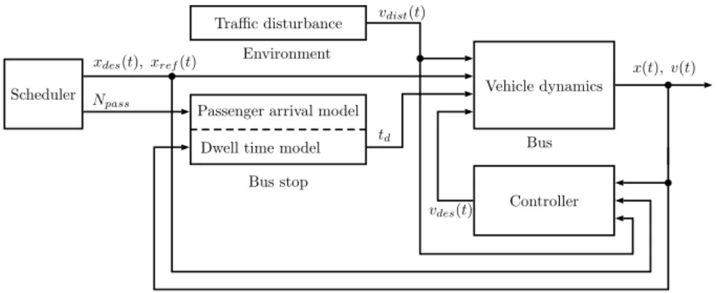
The velocity controller calculates a reference velocity profilevdesfor the bus based on two reference signals: (i) given the estimated dwell time and the sched- uled departure time from a stop, a desired trajectory is calculatedxdes(t); (ii) to keep equidistant headways, trajectory of the leading busxref(t) is also taken
100
into account. By means of balancing between these conflicting references, an optimal velocity profile is formulated. The proposed system can be classified as an overlapped, decentralized control. The controlled bus only requires the historical position of the leader bus and the schedule (stop locations and desired departure times), see Figure 1. In case either of them is missing or disabled,
105
the system can operate in either headway tracking or timetable tracking mode.
The control algorithm is generic, it can be applied to different routes, fleet con- figurations, schedules etc.
Place Figure 1 about here.
110
Figure 2 depicts the modularity of the proposed control system. Subsystems and notations are further detailed in the following parts.
Place Figure 2 about here.
3. Bus stop operations
This section presents the static models used for the bus bunching control
115
algorithm. The passenger arrival model in conjunction with the dwell time model describe the operations taking place at a bus stop. The control algorithm is deterministic, thus mean values are used for dwell time prediction. The predicted dwell time is used to estimate desired arrival times. The stochastic nature of the aforementioned models is exploited in the simulation scenarios,
120
bringing additional disturbances to the system. The scheduler is responsible for generating the reference signals for the buses.
3.1. Passenger arrival model
The average passenger waiting time at a stop can simply be described as half of the arrival rate of the public transport vehicle. This assumption holds
125
if the following conditions are fulfilled: passengers arrive randomly; passengers can get on the first arriving vehicle and vehicles have equal headways (Holroyd and Scraggs, 1966). In routes with frequent service (headways with 10 minutes or less) passengers typically do not consult schedules before arriving at their stops, their arrival rate can be thought random (Dessouky et al., 2003).
130
In (Jolliffe and Hutchinson, 1975) three types of passengers are categorized.
a) There are passengers whose arrival time is coincident with the bus.
These are the passengers who run to the stop because they see the bus coming, and thus wait zero time.
b) There are some passengers who plan their arrival at the bus stop so as
135
to be there just before the bus comes, minimizing their expected waiting time. This decreases the average waiting time (O’Flaherty and Mangan, 1970).
c) Finally, there are completely random passenger arrivals.
The arrival rate of groupb) andc) is described by Poisson distribution and their
140
ratio depends on the length of bus headways.
The time between successive arrivals is exponentially distributed with pa- rameterλ (arrival rate) and independent of the past. In the sequel, we use a Poisson distribution to inject passengers. However, we assume the hourly pas- senger demand at each stop Npass is known from the service provider. This
145
demand can be split into the three aforementioned categories. Figure 3 depicts the arrival rate of each passenger type between successive bus departures (tdep,i
andtdep,i+1). The area under the graph equals the number of passengers wait- ing at the stop. This is the number of boarding passengersPb which is used in the dwell time model.
150
Place Figure 3 about here.
3.2. Dwell time model
Dwell time is the average amount of time a public transport bus is stopped at the curb to serve passenger movements, including the time required to open and close the doors (Kittelson et al., 2003). Uncertainty in dwell times is a major
155
factor for bus bunching and it directly affects travel time and service quality.
The total time spent at stops can consume up to 26% of the total travel time (Rajbhandari et al., 2003). It is influenced by several factors: the configuration and occupancy of the bus, the number of boarding and alighting passengers, the configuration of stops, and the method of fare collection (e.g. on board or
160
pre-ticketing).
According to (Kittelson et al., 2003) time spent at a bus stop can be esti- mated knowing the number of boarding and alighting passengers, door configu- ration and other factors such as low floor, fare paying method etc. The average dwell timetd at a bus stop can be calculated as:
td=Pb·tb+Pa·ta+toc, (1) where
tb is the average boarding time per passenger, ta is the average alighting time per passenger, toc is the door opening and closing time,
165
Pb is the number of boarding passengers and Pa is the number of alighting passengers.
The boardingtb and alighting timeta of individual passengers can be modeled with normally distributed random processes. In the control design, average values are used: toc = 3.5 s, ta = 1.2 s and tb = 1.5 s, the dwell time is
170
proportional to the number of boarding and alighting passengers (Kittelson et al., 2003). Pb is obtained from the passenger arrival model (Section 3.1), the number of alighting passengers at each stopPa is considered to be known from the service provider.
3.3. Scheduler
175
Buses operate on a route based on a timetable. The scheduler, as a supervi- sor, defines where a bus shall be at a given time based on its timetablexdes(t).
Additionally, the reference position based on the leading busxref(t) is calcu- lated here. The timetable is static and obtained from the transport service provider in minutes resolution. For control design purposes this timetable was
180
refined to seconds.
4. Vehicle dynamics
The discrete-time model for the bus dynamics is based on the Optimal Ve- locity Model (OVM) (Bando et al., 1995). Position x(k), velocity v(k) and accelerationa(k) of a vehicle can be given as follows:
x(k+ 1) =x(k) +v(k)∆t, (2)
v(k+ 1) =v(k) +a(k)∆t, (3)
a(k) = 1
τ(vdes(k)−v(k)) (4)
where positionx(k+ 1) and velocityv(k+ 1) denote the states over the time period of [k∆t,(k+ 1)∆t] with discrete time step indexkand sampling time ∆t.
vdes(k) is the desired velocity at time stepk. τ is a model parameter capturing
185
the sensitivity of drivers to the change of their desired velocity. According
to (Helbing and Tilch, 1998) it shall be calibrated between 1.25 s and 2.5 s.
Too small values would result in rapid acceleration or deceleration towards the desired velocity. With autonomous vehicles these parameters could change, but still it is preferred to mimic the behavior of human drivers so their presence does
190
not perturb traffic significantly and does not disturb other drivers participating in traffic (Kesting et al., 2008).
The above equations can be written into state space form withvdes(k) being the controlled variable of the system: it serves as a display to the driver or a strict reference in case of autonomous driving. X(k) = [v(k), x(k)]T is the vector of system states at time step k. The state space representation of the system is therefore:
v(k+ 1) x(k+ 1)
=
1−∆tτ 0
∆t 1
v(k) x(k)
+
∆t τ
0
vdes(k). (5) 4.1. Traffic disturbance
An additive error structure is proposed to include the adverse effect of other vehicles participating in traffic. The control input vdes(k) is reduced as the average velocity decreases or traffic density increases on a link. Thus the velocity equation becomes:
v(k+ 1) =v(k) +∆t
τ (vdes(k)−v(k)−vdist(ρi, k)), (6) where vdist(ρi, k) is the velocity disturbance which is function of the traffic densityρi on linkiat time step k. The disturbance is included as a relaxation term with relaxation parameterβ ∈[0,1]:
vdist(ρi, k) =β(vdes(k)−vf und(ρi, k)). (7) β describes relaxation of bus speed towards a traffic dependent equilibrium velocity. With this term, road link specific obstacles such as traffic lights or
195
bottlenecks can be considered. The smallerβ is the slower vehicles adjust their velocity to the macroscopic velocity (Hoogendoorn and Bovy, 2001), (Van den
Berg et al., 2003). In Equation (7)vf und(ρi, k) denotes the macroscopic equi- librium velocity (Daganzo and Geroliminis, 2008) at linkiand time stepk. In the followings, for the sake of simplicity the argumentρi will be omitted from
200
vf und(k). Note that if the desired velocity falls below the equilibrium speed (vdes(k) < vf und(k)) the sign of the disturbance term changes. It forces the vehicle to increase its speed, in order not to delay traffic.
Substituting (7) into (6) results in the following velocity equation:
v(k+ 1) =v(k) +∆t
τ (vdes(k)·(1−β)−v(k) +β·vf und(k)). (8) If the bus travels on dedicated bus lane the disturbance term can be omitted by selectingβ = 0 or very small in Equation (8).
205
5. Reference speed control design
In this section the controller design process is outlined. First, the bus follow- ing model is augmented with two position references which shall be tracked by the controller. Then, the formulation of the optimization problem and the MPC design is presented. Next, different weighting strategies are proposed to enhance
210
timetable or headway reliability of buses. In addition, the Pareto Front of the two control objectives is formulated. Finally, three additional control strategies are outlined as benchmarks to the proposed controllers.
5.1. Reference tracking
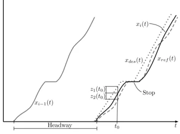
To ensure public transport service homogeneity, we propose a reference track-
215
ing controller. Set points are designed to increase public transport reliability both in time (schedule) and space (headway). The control algorithm shall ac- complish two objectives: timetable tracking and reduction of bus bunching. To this end, two error terms are introduced: z1andz2. z1(k) =xdes(k)−x(k) is the difference betweenxdes(k) (which is a reference position based on the timetable
220
and the estimated dwell time) and the actual position of the bus. The sec- ond error termz2(k) =xref(k)−x(k) denotes headway tracking (i.e. reducing
bunching). z2 is the difference between the actual position of the controlled vehicle and the shifted position of the leading bus. To minimize bunching, the trajectory of the leading bus is shifted by one headway and used as a reference
225
to the controlled vehicle, see Figure 4.
Place Figure 4 about here.
If the bus follows this trajectory, one headway distance is guaranteed in an insensitive way to the actual velocity of the leading bus. If the actual headway between the two buses is larger than the prediction horizon, the reference tra- jectoryxref(k) is known for every time iteration. (The leading bus has already traveled on that trajectory so this information exists.) The state space represen- tation of the system with the two performance outputs (reference trajectories) is as follows:
X(k+1)
z }| {
v(k+ 1) x(k+ 1)
=
A
z }| {
1−∆t
τ 0
∆t 1
X(k)
z }| {
v(k) x(k)
+
Bu
z }| {
∆t τ (1−β)
0
u(k)
z }| { vdes(k) +
Bς
z }| {
∆t
τ β 0 0
0 0 0
ς(k)
z }| {
vf und(k)
xdes(k) xref(k)
(9)
z(k)
z }| {
z1(k) z2(k)
=
C
z }| {
0 −1 0 −1
X(k)
z }| {
v(k) x(k)
+
D
z }| {
0 1 0
0 0 1
ς(k)
z }| {
vf und(k)
xdes(k) xref(k)
(10)
5.2. Shrinking horizon optimal control solution
230
The control oriented model is used as basis of a shrinking horizon MPC design (Maciejowski, 2002). The goal of the controller is calculating an optimal velocity profile between the actual position of the vehicle and the next stop, while taking into account several uncertainties, such as the adverse effect of traffic and randomness of dwell time. It is crucial to have accurate prediction for the dwell time and average traffic velocity. The desired arrival timetET Ais the scheduled departure timetET Dfrom the stop minus the modeled dwell time td (Section 3.1 and 3.2). (ET A and ET D stand for estimated time of arrival
and departure, respectively.)
tET A=tET D−td. (11)
A shrinking horizon strategy is chosen, where the horizon length is the estimated travel time to the next stop, see Figure 5. The interval between the actualt0and thetET A is split into N equidistant time samples to run the prediction model and perform the optimization. The initial horizon length of the controller N0
is calculated upon the bus departs from a stop: N0 = tET A∆t−t0. In every time
235
step the prediction horizon decreases by one. By the last time step the bus shall arrive the desired stop. To avoid small or even negative horizon lengths (due to lateness or being close to the stop) a lower boundary for the horizon length is defined: N =max{N, Nmin}, whereNmin= 5. Every subsystem in the model is discrete with the same sampling time, ∆t= 1s.
240
Place Figure 5 about here.
Consider the state space representation in Equation (9) and tracking per- formance Equation (10) and extend it forN horizon, see Equation (12). The system stateX(k) is measured at time stepk. Then, for a finite horizon length N the future statesX(k+i|k) are calculated along with the corresponding con- trol inputsu(k+i−1|k) and uncontrolled external input signalsς(k+i−1|k) . Predicted state is denoted asX(k+i|k), where time stepkat the right side within the parentheses denotes the current time, andkat the left side the pre- diction step with running indexi= 1,2, . . . , N. The same notation applies for
the control input the external signals and the performance outputsz(k+i|k).
ˆ x
z }| {
X(k+ 1|k) X(k+ 2|k)
.. . X(k+N|k)
=
A
z }| {
A A2 .. . AN
x
z }| { X(k) +
B
z }| {
Bu 0 · · · 0
ABu Bu 0
.. .
..
. . .. ... AN−1Bu AN−2Bu · · · Bu
u
z }| {
u(k) u(k+ 1|k)
.. . u(k+N−1|k)
+
E
z }| {
Bς 0 · · · 0
ABς Bς 0
.. .
..
. . .. ... AN−1Bς AN−2Bς · · · Bς
σ
z }| {
ς(k) ς(k+ 1|k)
.. . ς(k+N−1|k)
(12)
ˆz
z }| {
z(k+ 1|k) z(k+ 2|k)
.. . z(k+N|k)
=
C
z }| {
C 0 · · · 0
0 C 0
.. .
..
. . .. ... 0 0 · · · C
ˆ x
z }| {
X(k+ 1|k) X(k+ 2|k)
.. . X(k+N|k)
+
D
z }| {
D 0 · · · 0
0 D 0
.. .
..
. . .. ... 0 0 · · · D
ˆ σ
z }| {
ς(k+ 1|k) ς(k+ 2|k)
.. . ς(k+N|k)
(13)
Notations in Equation (12) are summarized below:
• X(k) is the vector of state variables: X(k) = [v(k), x(k)]T.
245
• Adenotes the state matrix.
• Bu is the control input matrix containing coefficients for the desired ve- locity: Bu= [∆tτ (1−β),0,0,0]T.
• u(k) is the controlled variable (decision variable). The only control input to the system is the desired velocity of the busu(k) =vdes(k).
250
• Bς is the coefficient matrix for the traffic disturbance.
• ς(k) is a vector, collecting the uncontrolled variables of the system, i.e. the disturbance from traffic flowvf und(k), the two references positions: xdes(k) andxref(k) at each time step.
ς(k) = [vf und(k), xdes(k), xref(k)]T.
255
• z(k) is the vector of performance outputsz(k) = [z1(k), z2(k)]T.
• C is the output matrix.
• D is the direct feedthrough matrix of the reference trajectories.
The cost-function can be formulated with the help of Equation (13) and Equation (12) in the following form:
J(k) = 1 2
hˆxT Qxxˆ+ˆzT Qzˆz+uT Rui
. (14)
ˆx,ˆzandudenote stacked vectors of the predicted states (velocity, position) performances (relative positions) and the control input (desired velocity) at each time step. The sole decision variable is the vector of desired velocities u over the prediction horizon. In every time step the initial states, disturbances and parameter matrices are frozen. Qx,Qz andRare diagonal, positive semi- definite weighting matrices:
Qx=
qv 0
0 qx
, Qz=
qx,des 0 0 qx,ref
, R=const ∈R1, (15) whereqv, qx, qx,ref andqx,ref are constant weights for their respective states.
In the MPC scheme these weights are also extended for N horizon: Qx =
260
diag(Qx, Qx, . . . , Qx)∈ R2N×2N, Qz =diag(Qz, Qz, . . . , Qz)∈R2N×2N, R = diag(R, R, . . . , R)∈RN×N.
A quadratic formula means that it penalizes both positive and negative de- viations from the reference (i.e. not only late but also early arrival). R adds cost to the control input. With some reformulation, the objective function to
265
be minimized becomes:
J(k) = 1 2uT
Φ
z }| {
BTQ
xB+BTCTQ
zC B+R
u+ (16)
+
ΩT
z }| {
xTATQ
xB+σTET Q
xB+xTATCT Q
zC B+σTETCT Q
zC B+ ˆσTDTQ
zC B u.
and we refer to detailed derivation in Appendix A. Finally, our control ob- jective
minu
1
2uTΦu+ ΩTu
, (17)
subject to:
|z1(k+N|k)|< ε, (18)
|z2(k+N|k)|< ε, (19)
vmin≤vdes≤vmax. (20)
In other words the two position errors shall be smaller thanε at the last time step. εis a tunable parameter in the inequality constraints, allowing a few me- ters tolerance. Furthermore, it is assumed that the control input is constrained:
270
the lower limitvmin = 0 km/h, since negative velocity is not allowed, vmax is constrained by the legal speed limit on the link (e.g. vmax= 50km/h).
The above optimization problem is an input constrained quadratic program- ming problem which can be solved with fast and efficient solvers (Nocedal and Wright, 2006). At the end of the optimization process,N control input signals
275
are obtained. This can be considered as an optimal velocity profile. However, only the first control inputu(k|k) is applied to the system. The process is then continued similarly by repeating the measurement, estimation, and optimiza- tion. Accordingly, the MPC is an online technique. Therefore, it is important to apply a sufficiently fast optimization tool and appropriate control interval.
280
5.3. Weighting strategies
In this section four different weighting strategies are proposed. The first is timetable tracking, where large weight is put on xdes relative to xref in the cost function. The second strategy is headway tracking, i.e. the goal is to mimic the trajectory of the leading bus. The third one is a balanced strategy
285
where timetable and headway references are equally important. Choosing the right control input weight is crucial. Finally, an adaptive strategy is presented incorporating varying control weights, depending on the magnitude of timetable and headway errors. If the control input is cheap (R is small) the control input resembles a bang-bang control strategy, most of the desired velocity valuesvdes
290
either vmin or vmax. If the control input is expensive (R is large), the system responds slowly and the desired performance criteria (timetable and headway
tracking) is not met. In other words, if R is large, demanding high velocity would result in high cost function values. Minimum of such a function would be at small control inputs over good performance.
295
The controller is tuned using the inverse square law (Bryson’s rule) (Bryson et al., 1979): the weights are normalized with the reciprocal of the maximum squared values of the states withQand the reciprocal of the maximum squared values of the control inputs withR.
Q=
q1
q2
. ..
qn
, R= 1
u2max (21)
with the elements inQbeing:
qi= γi
x2max,i, (22)
where qi, (the ith element of the diagonal) corresponds to the ith state in the state vector. Furthermore, γi is a tunable parameter, Pn
i=1γi = 1. In the nominator in Equation (22)xmax,i is the expected maximum value of the weighted state.
In the bus bunching control algorithmQis eitherQxorQmand the control
300
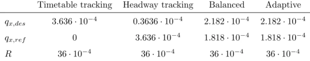
weights qi are defined as follows: {qv, qx, qx,des, qx,ref} for their respective states in the state vectorX(k) = [v, x]T and performance output vectorz(k) = [z1, z2]T. The weightRis related to the single control input, the desired velocity vdes. The corresponding weights for the four proposed control strategies are summarized in Table 1.
305
In every case the selected weight forqv is set to zero, because it would pe- nalize the kinetic energy of the bus (i.e. demand small velocity). Kinetic energy is weighted throughR. qx weights the absolute position of the bus. Minimiz- ing absolute position would be a physically unreasonable choice. Therefore the weights inQx are all zero, simplifying the cost function (see the Appendix A).
310
Next, an adaptive weighting strategy is proposed. This control strategy uses varying control weights based on the magnitude of timetable or headway errors.
Table 1: Control weights
Timetable tracking Headway tracking Balanced Adaptive qx,des 3.636·10−4 0.3636·10−4 2.182·10−4 2.182·10−4 qx,ref 0 3.636·10−4 1.818·10−4 1.818·10−4 R 36·10−4 36·10−4 36·10−4 36·10−4 By means of this adaptive weight selection it is possible to match headways more efficiently depending on the delay (timetable) and the level of bunching (headway). To this end a metric is introduced that describes the bunching level given by
ζ(k+i|k) =
z1(k+i|k) z2(k+i|k)
, (23)
where i = 1, . . . , N and ζ(k+i|k) ∈ [0, ζmax]. To apply this scaling other numerical considerations have to be taken into account: (i)ζis saturated with ζmax = 10 to avoid enormous control weights, (ii) to circumvent division by zero ζ = 1 if z2 = 0. The scaling parameter is calculated at the first step (upon departure from a stop) and frozen for the entire prediction horizon. It
315
is necessary to freeze the value of ζ in order to avoid algebraic loop in the solution. Thus, the optimization problem remains convex, see Appendix B.
With this scaling if headway errorz1is lowζ≈0, timetable schedule is tracked by means of weight selection. If there is a large deviation in headway, ζ 0, headway error will play dominating role in the cost.
320
The adaptive weighting matrix becomes:
Qz,adap(z1(k+i|k), z1(k+i|k)) =
ζ(k+i|k)·qx,des 0
0 qx,ref
. (24) It is sufficient to scale onlyqx,ref, since the ratio ofqx,ref andqx,desdetermine which objective is more important to track. In the adaptive weighting solution the same control weights are used as in the balanced strategy, see Table 1.
5.4. Pareto Front
The controller aims at striking a balance between headway and timetable
325
keeping. These two objectives do not have a unique solution but a set of op-
timal solutions. This set is called the Pareto Front (Veldhuizen and Lamont, 1998). With the Pareto analysis, we can quantify the gain of different weighting strategies.
In Section 5.3 weighting matricesQx,QzandRwere introduced. The MPC controller was obtained by minimizing a quadratic cost function. During this optimization, two objectives were taken into account: minimizing error relative to the headway of the leading bus and minimizing headway relative to the timetable. This optimization can be recast as a multiobjective problem. The weighting matricesQx,Qz andRare therefore decoupled as follows:
Qx
z }| {
qv
qx
=
Qx1
z }| {
αqv
αqx
+
Qx2
z }| {
(1−α)qv
(1−α)qx
, (25)
Qz
z }| {
qx,des
qx,ref
=
Qz1
z }| {
qx,des
0
+
Qz2
z }| {
0
qx,ref
, (26)
Furthermore,R is split too:
R=αR+ (1−α)R=R1+R2, (27) where α∈ [0,1] is a tradeoff parameter, i.e. when assuming equality between
330
the two performances α= 12. The control weights are extended to N horizon:
Qx1=diag(Qx1,1, Qx1,2, . . . , Qx1,N), Qx2=diag(Qx2,1, Qx2,2, . . . , Qx2,N), Qz1=diag(Qz1,1, Qz1,2, . . . , Qz1,N), Qz2=diag(Qz2,1, Qz2,2, . . . , Qz2,N),
335
R1=diag(R1,1, R1,2, . . . , R1,N) andR2=diag(R2,1, R2,2, . . . , R2,N).
The quadratic cost function can be reformulated with the help ofˆxandu:
J(k, N) =J1(k, N) +J2(k, N) = 1 2 h
ˆ
xTQx1xˆ+ˆzTQz1ˆz+uTR1ui +1
2 h
ˆ
xTQx2ˆx+ˆzTQz2ˆz+uTR2ui .
(28)
With the same deduction steps as in the single objective cost function (Equation (14) - (17)) the cost function becomes:
J(k, N) = 1
2uT(Φ1+ Φ2)u+ (ΩT1 + ΩT2)u. (29) The two sub-cost functionsJ1 and J2 will be used to demonstrate the Pareto Front. The methodology for obtaining the Pareto front is the following: from a selected initial statex,z and prediction horizonN an optimization is started using a genetic algorithm (Horn et al., 1994) with fixed control weights (headway,
340
timetable or balanced). Candidate solutions of the genetic algorithm with the lowest cost will form the Pareto Front.
5.5. Benchmark control strategies
To show the efficiency of the model predictive strategies three additional velocity control laws are developed.
345
Uncontrolled: Buses do not have any control applied to them, their desired velocity is the legal speed limit. They try to leave the bus stop as soon as possible.
Holding: Buses have no velocity control but they are held at stops until their scheduled departure time.
350
PI control: The PI (Proportional-Integral) controller uses the two refer- ence trajectories proposed in Section 5.1 but does not predict the desired trajectory as the MPC, only considers the actual timetable and headway tracking errorsz1(k) andz2(k) respectively. The control input for the PI controller is calculated as follows:
vdes,P I(k) =Pdes·z1(k)+Ides·
k
X
0
z1(k)+Pref·z2(k)+Iref·
k
X
0
z2(k), (30) withPdes= 0.025,Ides= 0.001,Pref = 0.025,Iref = 0.001 being tuning parameters for the PI controller with a balanced strategy. The controller was tuned using the Ziegler-Nichols method and also augmented with anti- windup due to the limitation ofvdes(Skogestad and Postlethwaite, 2005).
6. Simulation scenario
355
For comparative analysis a high-fidelity traffic simulator, VISSIM, is used (VIS, 2011). The simulator can be used to generate different traffic scenarios and evaluate the developed control algorithm.
Place Figure 6 about here.
360
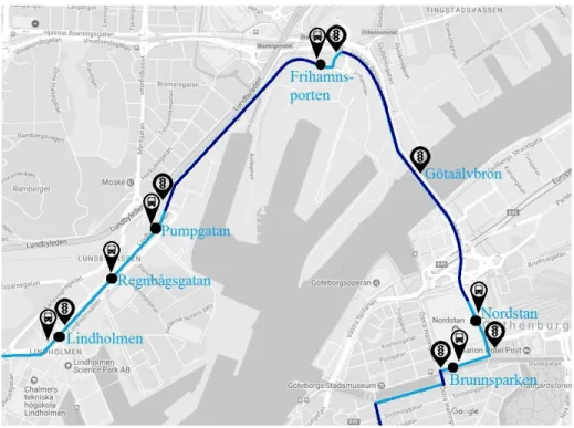
The route of Gothenburg’s trunk bus line 16 between Lindholmen and Brunns- parken is modeled, see Figure 6. The route is 4.3 kilometers long and includes six public transport stops. Between Lindholmen and Pumpgatan the line travels on a dedicated lane, then enters mixed traffic towards Frihamnsporten. On G¨ota
¨
alvbron it shares tracks with other public transport lines crossing the bridge
365
(e.g. tram line 5 and 6). Nordstan and Brunsparken stops are also shared with other lines. Buses have priority at signalized intersections, shown in Figure 6.
The legal speed limit is 50 km/h on the whole route. The time headway of the buses is 3 minutes. The passenger boarding and alighting volumes during peak hours at each stop is shown in Table 2. Furthermore, Table 2 summarizes the
370
total number of on-board passengers (in passenger per hour - not for individual vehicles) is summarized after each stop. In addition, the departure times from each stop is presented starting from Lindholmen stop at 0 seconds (repeating every 3 minutes).
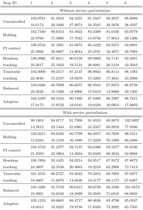
Table 2: Number of boarding and alighting passengers at each stop (passengers/hour), sched- uled departure time (seconds)
Boarding Alighting On-board Schedule
Lindholmen 1500 0 1500 0
Regnb˚agsgatan 600 75 2025 80
Pumpgatan 400 200 2225 160
Frihamnsporten 200 25 2400 330
Nordstan 400 600 2200 540
Brunnsparken 1500 1300 2400 720
The proposed vehicle to transport passengers on this route is a 18.75 meters
375
long, articulated bus. The passenger capacity is approximately 4 passengers per square-meter resulting in 135 persons passenger capacity. The ratio of standees and sitting passengers is not addressed.
During the simulations two types of disturbances are distinguished: (1) mi- nor disturbances coming from traffic lights, other vehicles and dwell time fluc-
380
tuation. (2) In order to investigate the control system under major disturbance, traffic flow is perturbed, vehicles are stopped in the middle of G¨ota ¨alvbron for ten minutes (i.e. opening the bridge). The simulator is capable of generating random boarding and alighting times, serving as an additional disturbance to the system. The models described in Section 3.1 and 3.2 are used to predict the
385
this behavior.
7. Simulation results
7.1. Bus trajectories
In the followings the proposed control algorithm is analyzed. The basis of the results is the simulation model presented in Section 6. First, one bus trajectory
390
with balanced control strategy is explained in detail, see Figure 7.
Place Figure 7 about here.
The blue circles represent the ideal departure times at each stop based on the bus schedule. The blue linexdesrepresents the ideal trajectory for timetable tracking. The red linexref is the trajectory of the leading bus, shifted by one
395
time headway (3 minutes). In this balanced strategy the follower (controlled) bus tries to minimize bunching (i.e. match the trajectory of the leading bus) and keep the timetable. For the next bus the reference headway will be the trajec- tory of the current bus. Eventually, the trajectories will converge to the original timetable while reducing bunching. The leading bus travels slowly between
400
Lindholmen and Regnb˚agsgatan (due to some disturbance). The controlled bus also slows down to avoid bunching. This results in lateness but it is recovered
by the end of the route. The bus holding strategy is also efficient in this sce- nario, the bus always departs from stops at the scheduled time instants but occupies stops for long periods. However, the bus holding cannot cope with
405
severe disturbances. Figure 7 also shows the timetable and headway errors at every time instant. The velocity profile of the bus is calculated by the shrinking horizon MPC controller. The control input is ranging betweenvmin = 0km/h and vmax = 50 km/h. The desired velocity profile is not followed accurately because the bus has its own dynamics plus it has to adjust its own velocity to
410
the surrounding traffic.
Figure 11 depicts the bus trajectories without velocity control where the desired speed of every bus is 50 km/h. The second bus enters the network with one minute delay (4 minutes headway). The blue circles represent the departure times at each stop based on the bus schedule. Since there is no
415
velocity control and the buses do not wait at stops till the scheduled departure time, their arrivals and departures are out of sync. This results in bunching too, see trajectory 2-3 in Figure 11. Another example is given without velocity control but with bus holding in Figure 12. This strategy can remedy bunching and adhere to the schedule at the cost of spending long times at the stop. For
420
example, Brunnsparken stop is almost always occupied by a bus.
The PI control can efficiently reduce bunching and adhere to the schedule with smaller computational demand than the MPC (Figure 13). However, it cannot cope well with disturbances: for example if the leading bus was stopped by a traffic light the controlled bus will also slow down regardless what the
425
traffic light indicates. On the other hand the MPC controllers consider a long trajectory ahead and buses can optimally adjust their velocity considering such obstacles (with the example of the traffic light - the MPC controller takes into account how long the leading bus was blocked by the traffic light).
Next, headway tracking MPC solution is implemented (Figure 14). With
430
this algorithm bunching is reduced, headway error is decreasing for consecu- tive buses. However, the buses are still out of sync with the schedule. The timetable tracking control strategy (Figure 15) can keep the schedule few head-
ways downstream the delay. Since the timetable is periodic, headway tracking is satisfactory too. The balanced control solution (Figure 16) has the best of
435
two worlds: the actual and reference trajectories overlap, meaning no bunching, while the timetable is kept too. The adaptive weighting method (Figure 17) can outperform the balanced control in both aspects. In the controlled simulations the first bus only obeys the timetable reference, headway reference does not exist.
440
7.2. Service recovery
In the following simulation scenario the response of each control strategy to extreme disturbance is evaluated. The traffic is stopped in the middle of G¨ota
¨
alvbron for ten minutes (i.e. opening the bridge). Over this period congestion is formed, delays increase. After, traffic is released and congestion starts to
445
dissipate. In the sequel, we analyze the metrics of service recovery from extreme perturbation. Here, we focus on congestion dissipation speed. In Figures 18-23 the space-time diagrams of the buses with different control strategies are shown.
The gray lines indicate a speed, thereof the the dissipation of congestion. It starts after the bridge is opened and vehicles start to queue up before Nordstan
450
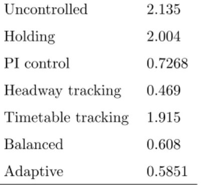
stop. The end point of the line shows when the vehicles arrive to Nordstan with the scheduled rate (headways recover to 3 minutes). The slope of the line is the dissipation speed of the congestion and is summarized in Table 3.
Table 3: Congestion dissipation speed (m/s)
Uncontrolled 2.135
Holding 2.004
PI control 0.7268
Headway tracking 0.469 Timetable tracking 1.915
Balanced 0.608
Adaptive 0.5851
In the uncontrolled and holding scenarios (Figure 18, 19) five buses are
affected by the service perturbation. The buses stopped at the bridge will re-
455
main bunched. Since there is no timetable or headway objective, vehicles leave the network as fast as possible, resulting in the fastest congestion dissipation.
As stated in (Newell, 1977), delays remain so high that the scheduling cannot recover from bunching. In order for the holding strategy to work in case of large disturbances, other measures, such as stop skipping, pulling out or insert-
460
ing buses shall be employed. The PI controller (Figure 20) can dissipate the congestion faster than the balanced controller but the system cannot recover well from the service perturbation, the buses leave the network bunched. With headway tracking strategy (Figure 21) bunching is completely eliminated but buses arrive with large delays at the next stop, not obeying the timetable. This
465
strategy results in slow service between the bridge and Nordstan stop in order to equalize headways. Congestion dissipation is very slow. Timetable tracking solution (Figure 22) cannot cope with the severe perturbation. The buses that got caught by the opening of the bridge stick together and cannot recover. The large difference between the desired trajectory based on the timetable and the
470
actual trajectory (i.e. large delay) forces the velocity controller to demand max- imum velocity. Therefore, in order to recover, another policy (e.g. slack times, stop skipping, dynamic timetable) has to be used. The scheduler does not make corrections due to perturbed service. The balanced technique (Figure 23) re- duces bunching compared to the timetable tracking but cannot eliminate it as
475
well as headway tracking. Recovery of the timetable takes more time compared to the timetable tracking policy. The trade-off between headway and timetable tracking can also be observed in the congestion dissipation speed. Finally, the adaptive weight approach (Figure 24) slightly outperforms the balanced control in terms of congestion dissipation. In this scenario, after releasing traffic at
480
the bridge both bunching and timetable reliability are poor (|z1| and |z2| are high). Since there is no way to adhere to the (static) timetable only headways are corrected gradually (z1 becomes small). Eventually, catching up with the timetable becomes more significant. In the multiobjective control approaches, given enough time both timetable keeping and bunching can be remedied.
485
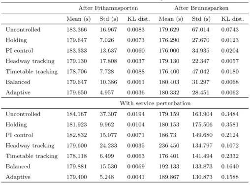
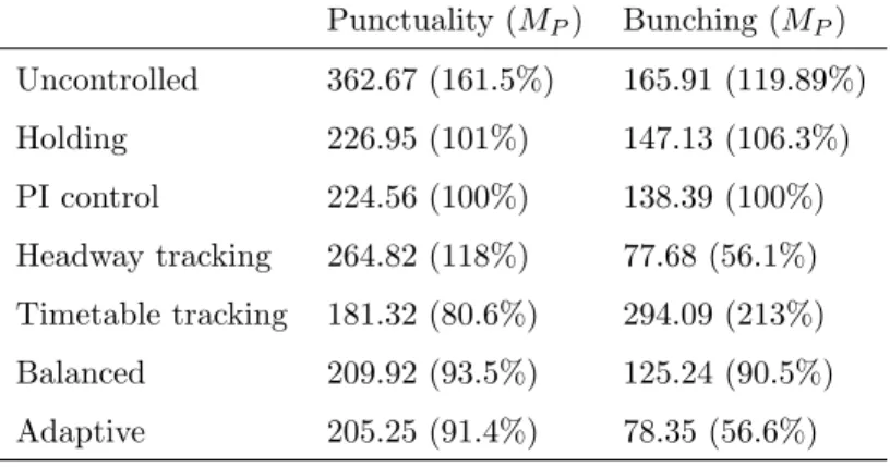
7.3. Headway reliability
Table 4 compares headway reliability in the different simulation scenarios based on statistical results: Headways are compared at two sections of the net- work: after Frihamnsporten and after Brunnsparken stops. The mean value is similar in every case, close to the ideal headway of 180 seconds (3min) except
490
for the headway tracking and balanced control strategies after the bridge was opened. The reason is that after the traffic is released from the bridge there is a huge headway gap between two buses which corrupts the mean value. On the other hand in those strategies where headway tracking is not addressed this huge gap is counterbalanced by the small headways of the congested buses. Further-
495
more, headway standard deviations are smallest in the headway tracking and balanced scenarios. Finally, the Kullback-Liebler (KL) divergence is given be- tween the ideal headway, and the simulation results, see (Kullback and Leibler, 1951). The ideal headway represents a uniform distribution with mean of 180 seconds and 0 variance. The KL distance is significantly smaller in the con-
500
trolled cases compared to the uncontrolled and the holding one after the service disruption, which means headways are more uniformly distributed. The PI con- trol works as well as the MPC solutions under in small disturbance conditions but performs significantly worse under major disturbance.
7.4. Average passenger waiting times
505
Average passenger waiting time relates directly to bus headways (Wu et al., 2017). If buses arrive irregularly, passenger waiting times will deviate more and the total waiting time will increase. Passenger arrivals at stops are generated by the simulator. In Equation (31) the average time passengers spend waiting for the bus at stopj is calculated. tdep,i−1andtdep,idenote the departure times of busi−1 and busi, respectively. Npass,j(k) is the number of passengers present at stopj at time stepkandNpass,j(tdep,i) is the terminal number of passengers boarding theith bus. ∆t= 1 is the sampling interval of the simulation.
T¯w,j =
tdep,i
X
k=tdep,i−1
Npass,j(k)∆t
Npass,j(tdep,i). (31)