Learning Based Approximate Model Predictive Control for Nonlinear Systems ?

(1)

Learning Based Approximate Model Predictive Control for Nonlinear Systems ?

D. Gángó^∗, T. Péni^∗ R. Tóth^∗∗

∗Systems and Control Laboratory, Institute for Computer Science and Control, Hungarian Academy of Sciences, H-1111 Bp. Kende u. 13-17.

(e-mail: gango.daniel@sztaki.mta.hu, peni.tamas@sztaki.mta.hu).

∗∗Eindhoven University of Technology, P.O. Box 513, 5600 MB Eindhoven, The Netherlands. (e-mail r.toth@tue.nl)

Abstract: The paper presents a systematic design procedure for approximate explicit model predictive control for constrained nonlinear systems described in linear parameter-varying (LPV)form. The method applies aGaussian process (GP) model to learn the optimal control policy generated by a recently developed fastmodel predictive control (MPC) algorithm based on an LPV embedding of the nonlinear system. By exploiting the advantages of the GP structure, various active learning methods based on information theoretic criteria, gradient analysis and simulation data are combined to systematically explore the relevant training points. The overall method is summarized in a complete synthesis procedure. The applicability of the proposed method is demonstrated by designing approximate predictive controllers for constrained nonlinear mechanical systems.

Keywords:model predictive control; Gaussian process; linear parameter-varying systems;

machine learning.

1. INTRODUCTION

Model predictive control (MPC) has several attractive features that make it an important control technology for engineering applications (Rakovic and Levine, 2019). For example, MPC can naturally handle strict state and input constraints and various performance specifications can be easily added to the design process. However, the price to be paid for these advantages is the high computational effort needed to obtain the control input: at every time instant a constrained optimization task has to be performed to get the next control action. This computational demand makes MPC less attractive for systems with fast dynamical components, e.g. mobile robots, aerospace applications and automotive systems. In order to apply predictive controllers to these model classes, the computational time has to be significantly decreased.

One approach to speed up the MPC is to compute the optimal control input as a function of the measured variables (e.g. as a function of the state if the state is available for measurement), store this function in memory and simply evaluate it during the control process. This strategy is called explicit MPC. If the optimization problem is linear or quadratic (this is the case if the system to be controlled is linear, the constraints are linear and the cost is linear or quadratic), the procedure that can be used to construct the parametric control function is multiparametric linear or quadratic programming (mpLP, mpQP), see e.g. Borrelli et al. (2019) for more details.

? This work was partially supported by the J´anos Bolyai Research Scholarship of the Hungarian Academy of Sciences and the ´UNKP- 18-4 New National Excellence Program of the Ministry of Human Capacities. It was also supported by the research program titled

”Exploring the Mathematical Foundations of Artificial Intelligence (2018-1.2.1-NKP-00008)”.

For nonlinear problems, the multiparametric optimization is currently under development (Johansen, 2003;

Dominguez et al., 2010), however, reliable solvers are not available yet.

This is where approximate solutions come into the pic- ture. Here the goal is to approximate the optimal control input up to some predefined tolerance. Theoretically, any function approximation method can be used, e.g., piecewise linear functions (Johansen, 2003), set member- ship methods (Canale et al., 2010), neural networks and machine learning (ML) solutions (Parisini and Zoppoli, 1995), (Csek¨o et al., 2015), (Hertneck et al., 2018). The latter methods are especially promising, because the resulting control laws can be efficiently implemented by using recently developed parallel software and hardware architectures, enabling applicability even for large-scale systems. As the approximation is independent of the un- derlying MPC algorithm, (it sees only the training data), this approach can be used for nonlinear MPC (NMPC) problems as well. Motivated by these attractive features of ML methods, the paper proposes a practical procedure for learning based approximate NMPC design. Compared to the other approaches, we put our focus on numerical efficiency: first, a fast nonlinear MPC algorithm based onlinear parameter-varying (LPV) embedding is applied to speed up the training point computation, second, a systematic procedure is proposed for exploring the most relevant training samples in order to improve the accuracy of the approximation while keeping the training set at a manageable size.

The paper is organized as follows. In Section 2 the LPV embedding based NMPC algorithm is introduced, while in Section 3, the concept of Gaussian process model based policy approximation is summarized. These are the

(2)

core components of the approximate MPC design method presented and analyzed in Section 4. The applicability of the proposed procedure is demonstrated in Section 5 on two application examples. The paper is finished with conclusions from the results achieved.

2. NONLINEAR MPC BASED ON LPV EMBEDDING This section presents the nonlinear MPC algorithm developed by H. Werner and his co-authors in Cisneros et al.

(2016). This algorithm is used to compute the optimal state feedback control policy that is then learned by a function approximator. The NMPC method is based on embedding of the nonlinear dynamics in an LPV model and applies iterativequadratic programming (QP)to solve the nonlinear optimization problem associated with the MPC synthesis. The algorithm is highly efficient as it has been demonstrated on moderate scale practical problems, although the convergence of the QP iteration has not been completely proven.

To begin, consider a nonlinear, discrete-time system rep- resented in an LPV form:

x_k+1=A(ρ(x_k))x_k+B(ρ(x_k))u_k (1) where kis the time index,xk ∈Rⁿ^x is the state,u∈Rⁿ^u is the control input and ρ(·) denotes the state-dependent scheduling parameter. For simplicity, we assume that the state is available for measurement. The control goal is to perform the standard regulation task, i.e., to steer the state from some initial value x₀ 6= 0 to the origin while minimizing a quadratic cost and satisfying a set of linear constraints prescribed for the state and input trajectory.

In the MPC setting this can be formalized by the following nonlinear optimization problem that has to be solved at each time instant to obtain the next control actionuk:

min

u_k|k, . . . uk+N−1|k

N−1

X

i=0

x^>_k+i|kQx_k+i|k+u^>_k+i|kRu_k+i|k+

+B(ρ(x_k+i|k))u_k+i|k (2b)

x_k|k=x_k (2c)

F x_k+i|k+Gu_k+i|k ≤h (2d)

x_k+N_|k ∈X_T (2e)

Here x_k+i|k, i= 0. . . N are the predictions of the future states based on the actual measurementxkand the control input sequenceu_k|k, . . . uk+N−1|k. Inequalities (2d) repre- sent the constraints,x^TW xandXT are the terminal cost and terminal set, respectively. The terminal ingredients used to ensure stability guarantees can be constructed by one of the several methods available in the literature.

A commonly used approach is to linearize the dynamics around the origin and construct the maximal ellipsoidal controlled invariant set for the linear system obtained. The details of this procedure are described, e.g., in Cannon et al. (2011).

To solve (2) Cisneros et al. (2016) proposes an iterative algorithm. In each iteration the parameter trajectory is fixed by using the state sequence obtained in the previous

step. This simplifies the dynamic model (2b) to a linear time-varying (LTV) system so the optimization problem can be solved by quadratic programming. The result is a new control input sequence. By applying this sequence on the nonlinear model, the next prediction of the state trajectory is obtained. The method is summarized in Algorithm 1.

Algorithm 1NMPC by LPV embedding Input:State vectorx, control horizonN.

Output:Control inputu

1: Let ¯x0= ¯x1=. . .= ¯xN−1=x

2: whilethe state and input trajectories do not converge do

3: Compute ¯ρ_i=ρ(¯x_i),i= 0, . . . , N−1.

4: Solve (2) with the LTV dynamics x_i+1=A( ¯ρ_i)x_i+B( ¯ρ_i)u_i,x₀=x.

The result is the optimalu^∗₀, . . . , u^∗_N₋₁ sequence.

5: Compute the state response of the nonlinear plant foru^∗₀, . . . , u^∗_N₋₁

¯

x_i+1=A(ρ(¯x_i))¯x_i+B(ρ(¯x_i))u^∗_i, fori= 0, . . . N−1, ¯x₀=x.

6: Letu=u^∗₀

It has been shown in Cisneros et al. (2018) that the iteration converges very quickly in practice: the stopping criterion is reached typically after 5-10 iterations. Since the procedure is based on quadratic programming, it requires much less computation time than a general nonlinear solver. This represents a serious advantage of Algorithm 1, compared to other NMPC methods in training set generation, where Algorithm 1 has to be performed several times with different initial states.

3. GAUSSIAN PROCESS BASED FUNCTION APPROXIMATION

Next, to obtain an explicit form of the control law repre- sented in Algorithm 1, we apply aGaussian process (GP) to approximate the general optimal control policy. GP, which represents a single layer based neural network, is chosen for this task, because it has a simple, expressive structure, that depends on relatively few tuning parameters and its training is fast and efficient. Moreover, GP provides information on the reliability of the approximation, which can be used to systematically select relevant training samples (active learning). A deep theoretical analysis of Gaussian processes can be found in Rasmussen and Williams (2006) while various engineering applications exploiting the attractive features of this structure are presented e.g. in (Liu et al., 2018), (Darwish, 2017), (Sharif, 2018), respectively.

From mathematical point of view, a GP is an infinite dimensional extension of the multivariate Gaussian distribution. Formally, a Gaussian processGP:Rⁿ →Ris a mapping that assigns to every pointx∈Rⁿa random vari- ableGP(x)∈Rsuch that for any finite setx⁽¹⁾. . . x^(M)the joint probability distribution ofGP(x⁽¹⁾), . . . ,GP(x^(M⁾) is Gaussian with meanmand covarianceK, where:

m= [m(x⁽¹⁾), . . . m(x^(M))]^T (3)

[K]ij =κ(xi, xj). (4)

Here [·]_ij denotes the (i, j)-th entry of a matrix andκis a suitable kernel function. (In the paper, we often use κ(·) with matrix arguments, so we may writeK=κ(X, X)).

(3)

Bothm(·) andκ(·) depend on additional tuning variables, denoted by θ. These are called the hyperparameters of the model. For given m(·) and κ(·) the sampling of the GP means sampling the Gaussian random variables at all x ∈ Rⁿ. The samples define a (deterministic) function g : Rⁿ →R, so the Gaussian process can be interpreted as a distribution over functions as well. If GP is used for regression, the goal is to learn a continuous function f :Rⁿ →Rby using a training set composed of (x, f(x)) tuples. The training is based on assuming that f is a sample of a GP and the goal is to find the most probable GP that can generate the training set. For this, the first step is the selection of the mean and kernel functions (model selection). By correcting the training data with its mean,m(·)≡0 can be chosen in general. It is thus enough to focus on the selection of the kernel function. The kernel is the core of the GP model. It determines the function class the GP is able to approximate. If the function to be learned is smooth and its characteristic length is almost constant, a simple Squared Exponential (SE) kernel is a good choice. On the other hand, if fast changes and discontinuities are expected, a more complex kernel, e.g. the Mat´ern class kernel has to be chosen. Further kernel functions with the related modeling capabilities are discussed in detail in Rasmussen and Williams (2006).

The next phase of the training is the tuning of the hyper- parametersθ. The most common learning rule is obtained by maximizing the marginal likelihood of the training samples. Specifically, ifT ={(x⁽¹⁾,y¯⁽¹⁾), . . . ,(x^(M⁾,y¯^(M⁾)}

is the training set and p(y|X, θ) withX = [x⁽¹⁾. . . x^(M⁾] denotes the M dimensional joint Gaussian distribution of GP(x⁽¹⁾). . .GP(x^(M⁾), then the goal is to maximize the marginal likelihood logp(¯y|X, θ) where ¯y = [¯y⁽¹⁾. . .y¯^(M⁾]^>. Since the gradient of logp(¯y|X, θ) inθcan be easily evaluated, a simple gradient ascent algorithm can be applied.

Now, assume that the GP has already been trained. An approximation of f at a test point x_∗ ∈ Rⁿ is obtained by taking the M + 1 dimensional joint distribution p([y⁽¹⁾, . . . , y^(M), y] | [X, x_∗], θ) and computing the one dimensional conditional distribution p(y|x_∗, y⁽¹⁾ =

¯

y⁽¹⁾, . . . y^(M⁾= ¯y^(M), X, θ). The meanm_∗ of this distribution is considered to be the approximation forf(x_∗), while the varianceσ_∗ provides information on the uncertainty of the regression. As all distributions above are Gaussian, the evaluation of a GP requires only elementary matrix manipulations so it can be performed efficiently.

4. ACTIVE LEARNING OF APPROXIMATE MPC POLICY

4.1 Outline of the concept

In many safety critical mechatronic and automotive applications, it is highly important to ensure deterministic computation time of the control law under a fast sampling rate. Even if Algorithm 1 has one of the fastest solution times, its rate of convergence to an optimum is problem dependent. Hence, to enable reliable real-time execution of the LPV MPC method, we intend to construct an approximate controller that is much faster to evaluate online and has a deterministic execution time. For this, a training set T = {(x⁽¹⁾, u⁽¹⁾), . . . ,(x^(M⁾, u^(M))} is generated by performing Algorithm 1 M times with initial

valuesx⁽¹⁾. . . x^(M⁾and then a GP is trained by using this data to learn the optimal control policy.

A crucial part of training is to select the most relevant training samples and keep the size M of the training set minimal. This gives rise to the need for a systematic method for exploring the most informative training points that help to reduce the approximation error.

Along with the results presented in Krause et al. (2008), Brochu et al. (2010) and Boef, den P. (2019) we apply the following method for training point selection. First the training set is initialized, then active learning methods are applied to select additional training points. Finally, the training set is refined by controlling the system such that both the NMPC and the approximated control inputs are simultaneously computed at each time instant. The points where the GP performs poorly compared to the NMPC are added to the training set. Note that the simultaneous control can be implemented in simulation, or on a real plant provided that a suitably powerful computing device is available to run the NMPC and GP in real time. Of course, after the required level of precision is reached, the online NMPC can be removed from the loop. This can be seen as a procedure of tuning in a laboratory environment before the approximate MPC can be deployed on the real system.

4.2 Step I: Initial training set generation

Let (X,U) denote the admissible input and state space.

Moreover, let V ⊂ X denote a set of discrete samples, the potential places of training points. A straightforward way to specify V is to generate a dense, equally spaced grid over the state space, but it can be also generated by random sampling as well. The initial training set T0

can be determined in two different ways. One approach is to randomly draw entries from V, and calculate their corresponding input values using the NMPC algorithm.

The other, more structured method is to get the instances ofVwhich lay on a sparse, equally spaced grid of the state space. In the sequel, we will denote byAall the points ofV that are present in the training setT. The complementer setV\A, collecting the free points is denoted by ¯A.

4.3 Step II: Active learning based training point generation Once the initial training setT₀ has been generated, additional training points are selected from ¯A, to reduce the approximation error of the GP. In this phase, we want to ensure that each point selected decreases the most the global approximation error reduction of the GP with respect to the control policy. For this purpose, 3 training point selection methods are proposed. They can be used individually, or at the cost of computational complexity can be combined to achieve better performance.

Maximum gradient: It is straightforward to assume that the more abruptly the approximated function changes, the more training points are needed for its accurate approximation. Therefore, the gradient of the mean function of the GP can be used as a query function to the training point selection. In case of one test pointx_∗, the gradient of the mean function is

∇f¯x∗=∇k^>_∗K_A⁻¹y, (5)

(4)

where XA =

x⁽¹⁾ x⁽²⁾ . . . x^(M⁾>

is a matrix assembled from the elements of A, y =

y⁽¹⁾ y⁽²⁾ . . . y^(M)^>

is the vector of input values corresponding to the elements ofA, k∗ = κ(XA, x∗) is the vector of covariances between the test pointx_∗and the points inA, andK_A=κ(X_A, X_A) is the covariance matrix of the points inA. After the gradient has been calculated for each potential training point in ¯A, we calculate the norm of the gradients, and choose the point with the highest gradient norm to be added to the training set.

Maximum variance: Besides the predictive mean, the variance can be also calculated for anyx_∗test point. The variance is an indicator of the uncertainty of the GP, and thus is a suitable query function for training point selection. According to Rasmussen and Williams (2006), for a single test point the variance can be written as

σ²_x_∗_|A=κ(x_∗, x_∗)−k^>_∗K_A⁻¹k_∗. (6) Similarly as before, the potential training points can be ranked based on their variance values, and the one with the highest variance is added to the training set.

Mutual information: In the training point selection process, our goal is to select the element ofAsuch that it reduces the uncertainty of the predictions in ¯A the most.

According to Krause et al. (2008), this is equivalent to finding the setAthat maximizes the mutual information MI(A) = I(A,A). Using a greedy selection approach,¯ we sequentially choose the points which maximize the increment of the mutual information

arg max

x∈A¯

MI(x∪ A)−MI(A), (7) This can be simplified to

arg max

x∈A¯H(x|A)−H(x|A),¯ (8) where H(x|A) is the entropy of x conditioned on the elements ofA, and can be expressed as a function of the variance,

H(x|A) =1

2log(σ²_x|X_A) +1

2(log(2π) + 1). (9) The calculation is analogous forH(x|A) with the replace-¯ ment of A with ¯A. For the details of the derivation and the technical aspects of the selection algorithm see (Krause et al., 2008).

Note that it is possible to use these selection concepts by themselves, but the combined use of them with ap- propriately chosen weights (w_v, w_g, w_mi)≥0,w_v+w_g+ wmi = 1 can be also beneficial. The pseudo-code of the active learning algorithm is summarized in Algorithm 2.

A comparison of different selection methods is shown in Figure 1.

4.4 Step III: Control refinement in closed loop

After the augmentation of the training set it is still possible that at certain points of the state space the approximation error of the GP exceeds the allowed tolerance. (In our algorithm, the threshold is set a-priori by analysing the robustness properties of the NMPC algorithm.) To ensure that all the control relevant points are included in the training set, we propose the following refinement strategy. First, a large number of initial states are generated randomly within the bounds of the state constraint. For each initial

Algorithm 2 Training point selection by using active learning

Input:Gaussian process model GP, training setT, set of potential and current training point locations ¯A,A, weigths wv, wg, wmi, number of training points to be addedj

Output:GP,T

1: fori= 1 toj do

2: forx∈A¯do

3: δ^v_x←σ_x|A²

4: δ^g_x← ∇f¯x 5: δ^mi_x ←σ_x|A² /σ²_x|_A_¯

6: δ_max^v ←max_x∈A¯δ_x^v

7: δ_max^g ←max_x∈A¯δ_x^g

8: δ_max^mi ←max_x∈A¯δ_x^mi

9: x∗←arg max_x∈A¯(wvδ_x^v/δ_max^v +wgδ_x^g/δ^g_max+ +wmiδ^mi_x /δ_max^mi )

10: A ← A ∪x_∗

11: A ←¯ A\x¯ ∗

12: uMPC←calculate optimal MPC input for x∗ 13: T ← T ∪(x∗, uMPC)

14: GP←retrain GP withT

150 200 250 300 350 400 450 500

number of training points 0.02

0.04 0.06 0.08 0.1 0.12 0.14 0.16

mean absolute error

variance (random initial set) variance

mutual information (random initial set) mutual information

variance and gradient norm mutual information and gradient norm 55% varance and 45% gradient norm

Fig. 1. The comparison of various active learning methods and their effect on the global absolute mean approximation error computed onV. The criterion functions to be maximized are indicated in the legend for each curve. The curves with solid lines share the same initial training set with training points placed on an equidistant grid, whereas the curves with dashed lines also share an initial training set with randomly placed training points.

state, the system is simulated until it reaches the terminal set. During the simulation, both the NMPC algorithm and the GP are evaluated to calculate both the optimal input valueuMPC and its approximationuGP. At each step the difference of the optimal and the approximated input is checked: if it exceeds a certain thresholdε, then the current state and optimal input pair (x, uMPC) is included in the training set and the GP is retrained. After a sufficient number of simulations, this method should result in a GP model with a finalized training set, which is able to fulfill the control task with near-optimal control inputs (within the specified tolerance bounds). Guaranteed robustness against the approximation error can be achieved by choos- ing a suitable small tolerance ε and applying constraint

(5)

tightening in the MPC design. One possible procedure is proposed in Hertneck et al. (2018). The pseudo-code of the refinement method is summarized in Algorithm 3.

Algorithm 3 Control oriented learning with simulation data

Input: Gaussian process model GP, training set T, system matricesAandB, terminal set, error tolerance ε, number of simulationsj

Output:GP,T

1: fori= 1 toj do

2: x←assign random value within constraints

3: T+←initialize empty set

4: whilexis outside the terminal setdo

5: uMPC ←calculate optimal MPC input

6: uGP←infer GP at test pointx

7: if |uMPC−uGP| ≤εthen

8: u←uGP

9: else

10: T+← T+∪(x, uMPC)

11: u←uMPC

12: x←Ax+Bu

13: T ← T ∪ T+

14: GP←retrain GP with the new training set 5. APPLICATION EXAMPLE: CONTROL DESIGN

FOR A SIMPLIFIED HELICOPTER MODEL In this section the approximate NMPC design procedure is presented on an application example.

Consider the simplified 2D helicopter model from Cannon et al. (2011).

¨

y= (u₁+g) sin(α), z¨= (u₁+g) cos(α)−g, α¨ =u₂ (10) where y, z and α denote the position and orientation of the helicopter. The net thrust and moment acting on the helicopter are proportional to the inputs u1 and u2, respectively. The control task is to drive the helicopter from any arbitrary initial hovering state x0 = [y0 z00 0 0 0]^>

to the terminal set placed at the origin. The constraints of the system are|y| ≤1, |z| ≤1, |y| ≤˙ 0.5, |z| ≤˙ 0.5, |α| ≤ 0.3, |α| ≤˙ 0.5, |u1| ≤10, |u2| ≤10, with cost weight ma- trices Q= diag(0.1,0.1,1,1,10,1), R= diag(10⁻⁴,10⁻³).

The LPV form of the system is formulated as







˙ y

˙ z

¨ y

¨ z

˙ α

¨ α







=







0 0 1 0 0 0 0 0 0 1 0 0 0 0 0 0 gρ1 0 0 0 0 0 gρ₂ 0 0 0 0 0 0 1 0 0 0 0 0 0











 y z

˙ y

˙ z α

˙ α





 +





 0 0 0 0 ρ3 0 ρ₄ 0 0 0 0 1





 u1

u₂

= (11)

=A(ρ)x+B(ρ)u, ρ1= sin(α)

α , ρ2=cos(α)−1

α , ρ3= sin(α), ρ4= cos(α).

For control design, the continuous model was discretized by Euler’s method:

x_k+1= (I+hA(ρ_k))x_k+hBu_k, (12) whereh= 0.1 s is the sampling time. In the GP model, due to the expected discontinuities of the explicit MPC law, a Mat´ern class kernel was used (Rasmussen and Williams (2006)), namely

κ(x_p, x_q) =σ_f²(1 +√

3r) exp(−√

3r), (13) r= (xp−xq)^>M(xp−xq),

whereM = diag(l_i⁻²), i= 1, . . . ,6 andσf, l1, l2, . . . l6 are the hyperparameters of the model.

Since the system has 2 inputs, two separate GP models were required for the approximation, however, during our calculations we used one common training set for the two models.

First, a validation set was constructed to be used for qualifying the approximation. For this, we calculated the optimal input values on an equidistant grid with 0.1 spacing from−1 to 1 inyandz, and with constant 0 in the other 4 state variables. We also included in the validation set all the states along the predicted trajectories with their corresponding input values on anN = 30 prediction horizon obtained from the NMPC algorithm. This resulted in a set that fairly represents all the states the system can reach while executing the control task.

Then the set of potential training point locations V was obtained by gridding the whole state space (with 0.2 spacing along all 6 dimensions) and selecting only those points that lay inside the convex hull of the points in the validation set. The initial training set was assembled by using a sparser grid with 0.5 spacing along y and z and 0.2 spacing along the remaining 4 dimensions. This resulted in 257 initial training points. Afterwards, the active learning algorithm increased the number of training points to 945. The selection criteria were the maximum variance and the maximum gradient norm, with weights wv = 0.55 and wg = 0.45, respectively. In each iteration, one point was selected for each GP, and both points (if different), were added to the same, shared training set.

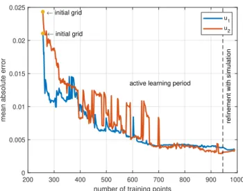
Finally, the refinement process with tolerance ε = 0.1 increased the number of training points to 990. Figure 2 shows the average absolute error of the approximations during the training process, compared to the validation set described earlier. Figure 3 shows that the GP models were able to learn the control input. In the figure, 500 trajectories are shown which were generated by controlling the system with the fully trained GPs alone.

During the simulation the average runtime of the 2 GP’s inference together was 0.2321 s, whereas the average runtime of the NMPC algorithm was 1.1880 s. This shows, that after a certain level of system complexity, the real time evaluation of the NMPC algorithm becomes in- tractable, while the time required to GP inference does not increase significantly.

Finally, the GP regression was compared with linear interpolation. The interpolation was evaluated on the same dataset over which the GP is defined. By examining the control performance from the 500 initial conditions depicted in Fig. 3, we found that GP performed better in several aspects: first, the computation of the control input by interpolation was approximately 20 times slower compared to the GP (we used the built-in interpolation routines of Matlab). Second, the dataset was proved to be inadequate for linear regression: in some cases the linear interpolation produced high approximation error resulting in poor control performance or unstable closed- loop behavior.

6. CONCLUSION

In this paper a practical approach is presented for con- structing a learning based approximate explicit LPV

(6)

200 300 400 500 600 700 800 900 1000 number of training points

0 0.005 0.01 0.015 0.02 0.025

mean absolute error

initial grid

active learning period

refinement with simulation

u₁ u₂

Fig. 2. The average absolute error of the approximation of the optimal input for the helicopter, compared to the validation set. The jumps in the average absolute error ofu2 are the result of the parameters in the GP model converging to different local optima during the training.

-1 -0.8 -0.6 -0.4 -0.2 0 0.2 0.4 0.6 0.8 1

y -1

-0.8 -0.6 -0.4 -0.2 0 0.2 0.4 0.6 0.8 1

z

Fig. 3. Trajectories of the helicopter model controlled using the GP based explicit controller from random initial statesx0= [y0 z0 0 0 0 0]^> to the terminal set.

model predictive controller for nonlinear systems. Special attention is paid to the systematic collection of relevant training samples. It has been shown that active learning methods and closed loop simulations can be successfully blended in an efficient training point selection algorithm.

The applicability of the procedure has been demonstrated by designing an approximate predictive controller for a nonlinear mechanical system.

REFERENCES

Boef, den P. (2019).Frequency Domain LPV System Iden- tification Using Local Data. Master’s thesis, Eindhoven University of Technology.

Borrelli, F., Bemporad, A., and Morari, M. (2019).Predic- tive Control for Linear and Hybrid Systems. Cambridge University Press.

Brochu, E., Cora, V.M., and Freitas, N.D. (2010). A tutorial on Bayesian optimization of expensive cost

functions, with application to active user modeling and hierarchical reinforcement learning. arXiv:1012.2599.

Canale, M., Fagiano, L., and Milanese, M. (2010). Effi- cient model predictive control for nonlinear systems via function approximation techniques. IEEE Transactions on Automatic Control, 55(8), 1911–1916.

Cannon, M., Buerger, J., Kouvaritakis, B., and Rakovic, S. (2011). Robust tubes in nonlinear model predictive control. IEEE Transactions on Automatic Control, 56(8), 1942–1947.

Cisneros, P.S.G., Sridharan, A., and Werner, H. (2018).

Constrained Predictive Control of a Robotic Ma- nipulator using quasi-LPV Representations. IFAC- PapersOnLine, 51(26), 118–123.

Cisneros, P.S.G., Voss, S., and Werner, H. (2016). Efficient Nonlinear Model Predictive Control via quasi-LPV Rep- resentation. InProceedings of Conference on Decision and Control, 3216–3221.

Csek¨o, L.H., Kvasnica, M., and Lantos, B. (2015). Explicit MPC-Based RBF Neural Network Controller Design With Discrete-Time Actual Kalman Filter for Semiac- tive Suspension.IEEE Transactions on Control Systems Technology, 23(5), 1736–1753.

Darwish, M.A.H. (2017). Bayesian identification of linear dynamic systems. Ph.D. thesis, Eindhoven University of Technology.

Dominguez, L.F., Narciso, D.A., and Pistikopoulos, E.N.

(2010). Recent advances in multiparametric nonlinear programming. Computers & Chemical Engineering, 34(5), 707–716.

Hertneck, M., K¨ohler, J., Trimpe, S., and Allg¨ower, F.

(2018). Learning an approximate model predictive controller with guarantees. IEEE Control Systems Letters, 2(3), 543–548.

Johansen, T.A. (2003). Approximate explicit receding horizon control of constrained nonlinear systems. Au- tomatica, 40(2), 293–300.

Krause, A., Singh, A., and Guestrin, C. (2008). Near- optimal sensor placements in Gaussian processes: The- ory, efficient algorithms and empirical studies. Journal of Machine Learning Research, 9(Feb), 235–284.

Liu, M., Chowdhary, G., da siLva, B.C., Liu, S., and How, J.P. (2018). Gaussian Processes for Learning and Control - A tutorial with examples. IEEE Control Systems Magazine, 38(5), 53 – 86.

Parisini, T. and Zoppoli, R. (1995). A receding-horizon regulator for nonlinear systems and a neural approximation. Automatica, 31(10), 1443–1451.

Rakovic, S.V. and Levine, W.S. (eds.) (2019). Handbook of Model Predictive Control. Birkh¨auser.

Rasmussen, C.E. and Williams, C.K.I. (2006). Gaussian Processes for Machine Learning. MIT Press.

Sharif, B. (2018). Linear Parameter Varying Control of Nonlinear Systems. Master’s thesis, Eindhoven Univer- sity of Technology.