On the Effects of Strong Asymmetries on the Adaptive Controllers Based on Robust Fixed Point
Transformations
Kriszti´an K´osi (PhD student)
Doctoral School of Applied Informatics Obuda University´
Budapest, Hungary Email: krisztian.kosi@gmail.com
J´anos F. Bit´o, J´ozsef K. Tar Institute of Applied Mathematics
Obuda University´ Budapest, Hungary
Email:
{bito@, tar.jozsef@nik.}uni-obuda.hu
Abstract—For replacing Lyapunov’s sophisticated “2nd Method” in the design of adaptive controllers a novel approach based on Robust Fixed Point Transformations (RFPT) was pro- posed that directly concentrates on the designer’s intent instead of forcing global stability. It guarantees convergence only in a bounded basin while iteratively generating the sequence of the appropriate control signals. In the initial phase of this iterative learning considerable fluctuation may occur in the control signal that otherwise may be limited due to phenomenological reasons.
While in mechanical systems positive or negative force or torque components can be allowed, in controlling chemical reactions negative ingress rates of pure reactants into a stirring tank reactor phenomenologically cannot be realized. While velocity components may have well interpreted positive or negative values, negative concentrations physically cannot make sense. On this reason the mathematical models of chemical reactions normally containing the products of various powers of the concentrations must be completed with truncation-type nonlinearities that intro- duce strong asymmetric nonlinearities. In this paper the effects of these phenomena are investigated via computer simulations in the adaptive control of a Classical Mechanical and a chemical system. It was found that in spite of these limitations the adaptive controller can still work at least in certain segments of the whole control section.
I. INTRODUCTION
In the adaptive control ofClassical Mechanical Devicesas robots and various manipulators usually we have to cope with strongly coupled nonlinear equations of motion the solution of which does not have closed analytical form. For studying their solutions the use of purely numerical techniques cannot be satisfactorily applied since the validity of their results are restricted only to the time interval of the actual investigations.
In general no reliable extrapolation for +∞ in time can be done on the basis of computations. On this reason the ingenious method invented and published by Lyapunov in his PhD dissertation in 1892 [1] became the almost only essential tool for designing globally stable controllers for nonlinear systems. Translations of his work to English (e.g. [2]) and French appeared in the middle of the past century well inspired the development of control technology.Its main virtue is that without knowing the details of the behavior of the solution
its stability can be determined or granted on the basis of relatively simple estimations that can be carried out even in analytical form. Both model-based predictive controllers as well as their adaptive variants as the Adaptive Inverse Dynamics Controlleror theSlotine-Li Model-Based Controller and its adaptive variants (e.g. [3], [4], [5]) intensively use this technique. While these controllers try to adaptively tune the parameters offormally exactly known models of approximately available parameters, another class of the adaptive controllers, the so called Model Reference Adaptive Controllers (MRAC) rather apply this technique for generating fast control signals that make the behavior of the controlled systems similar to that of areference system normally having far more “decent”
dynamical properties as the actual one under control (e.g.
[6], [7], [8], [9]). The Lyapunov function technique is widely use in the design of Robust Variable Structure/Sliding Mode Controllers, too (e.g. [10]).
Though the fact of global stability guaranteed by this method is very important, other important design goals as precise prescription of the relaxation of the tracking errors cannot directly met by this technique. For properly setting the arbitrary control parameters that normally are present in a great number in the case the Lyapunov function based techniques (mainly in the free parameters of the big positive definite symmetric matrices) ample amount of computations are needed normally by the application evolutionary methods to meet the primary design goals (e.g. [10], [11], [12]).
Another drawback of the Lyapunov function-based techniques that they need designers having excellent skill in Mathematics.
The proofs of convergence usually consume up several pages in the appropriate papers. These drawbacks of Lypunov’s technique motivated seeking alternatives that gave up the need for global stability in order to bring the primary design goals in the foreground on the basis of far simpler considerations. The essence of these methods is briefed Section II. The usability of these new methods were extensively investigated in the adaptive control of Classical Mechanical systems and certain chaotic systems as certain neuron models as e.g. [13], and
the hydrodynamic model of freeway traffic [14]. However, up to now little if any effort was done to investigate the application possibilities for the control of chemical reactions.
In the present paper the case of theBrusselator Model of the The Belousov-Zhabotinskii Reactionwill be considered, too.
II. ADAPTIVECONTROLUSINGROBUSTFIXEDPOINT
TRANSFORMATIONS
The mathematical principles of the application of the RFPT transformations in adaptive control were expounded in details e.g. in [15]. The application of the same idea within the novel mathematical structure of MRAC controllers also was explained in details e.g. in [16]. Appropriate variants were developed forSingle Input - Single Output (SISO)andMultiple Input - Multiple Output (MIMO) systems, too. Since in this paper only MIMO systems are considered, the basics of this method are briefly summarized on the basis of [15] and [16]
as follows.
This approach can be applied in control tasks in which the controlled response of the physical system under control is directly measurable and no model-base filtering technique (e.g.
some Kalman Filter [17]) must be used for state estimation.
In the case ofdynamic systemsthissystem response normally corresponds to certain time-derivatives of the state variables: in Classical Mechanics for fully driven systemsit corresponds to
¨
𝑞, i.e. the 2nd time-derivative of the generalized coordinates; in chemical reactionsto thetime-derivative of certain concentra- tions. For driving the system through a set of time-dependent states (depending on the system’s phenomenology) a desired response𝑟𝑑can be prescribed by the designer of the controller.
This desired response normally makes the system’s actual state asymptotically converge to the prescribednominal value.
Normally, in the lack of precise system model the designer applies some available approximate model to calculate the appropriate “physical agents” that can bring about the desired response. In mechanical systems these agents are force or torque components, in chemistry they correspond to some ingress rate of certain reagents that are fed into the reaction vessel. Due to the imprecisions in the model, the actually applied “agents” bring about a realized response 𝑟𝑟:=𝑓(𝑟𝑑) that differs from the desired one: 𝑟𝑟 ∕=𝑟𝑑. In this cases the
“response function”𝑓()can evidently be introduced. Though its analytical form is not known, this function is known in the sense that its input value is known, and its output value is measurable. Instead of trying to tune the parameters of the imperfect (and frequently also incomplete) model in order to obtain the ideal 𝑟𝑟 ≡ 𝑟𝑑 response function the RFPT- based approach constructs a contractive mapping by the use of which in each control cycle an element of a convergent sequence of inputs to the approximate model, the sequence of the “required” responses{𝑟𝑛} is generated that converges to the solution of the control task, i.e. 𝑟𝑛 → 𝑟★ so that 𝑓(𝑟★) =𝑟𝑑. In [15] the details of the convergence were also expounded.
The application of the same idea in the case of MRAC controllers was explained in [16]. The essence of MRAC int
his view is that external, and internal control loops are so applied that the external loop computed the desired response on purely kinematical basis and it calculates the appropriate model of a perfectly knownreference system. Evidently, since the reference system considerably differs from the actual one, an internal control loop deforms this reference force before applying it on the actual system to obtain the desired response.
Finding this proper deformation now happens in the space of the forces by convergent sequence of the “required forces”
that are generated by similar RFPT transformations. When this sequence well approaches the appropriate one causing the desired response the external loop has the illusion that by the application of the dynamic model of the reference system it can obtain precise tracking, i.e. the “MRAC illusion” is brought about. In the case of SISO systems the appropriate sequences were generated by the function given in (1)
⃗ℎ𝑛+1:= ⃗𝑓(⃗𝑟𝑛)−⃗𝑟𝑑𝑛+1, ⃗𝑒𝑛+1:=⃗ℎ𝑛+1/∣∣⃗ℎ𝑛+1∣∣, 𝐵˜𝑛+1=𝐵𝑐𝜎(𝐴𝑐∣∣⃗ℎ𝑛+1∣∣),
⃗𝑟𝑛+1= (1 + ˜𝐵𝑛+1)⃗𝑟𝑛+ ˜𝐵𝑛+1𝐾𝑐𝑂⃗𝑒𝑛+1
(1)
in which 𝜎(𝑥)a smooth, strictly increasing function varying between ±1 also satisfying the additional restrictions that 𝜎(0) = 0, and 𝑑𝜎𝑑𝑥∣𝑥=0 = 1. In the close vicinity of the fixed point in which∣∣⃗ℎ𝑛+1∣∣is very small (i.e. if∣∣⃗ℎ𝑛+1∣∣< ℎ𝑙𝑖𝑚𝑖𝑡), instead of the use of the mathematically near singular normal- ization the ⃗𝑟𝑛+1 := ⃗𝑟𝑛 rule can be applied. The numerical value of ℎ𝑙𝑖𝑚𝑖𝑡 may depend on the typical numerical range of the particular control application under consideration. The new element first published here is the introduction of the orthogonal matrix𝑂 that can modify the direction of the unit vector along which that adaptive deformation is applied. (In the former applications only the case𝑂≡𝐼was investigated.) Apart from the orthogonal matrix𝑂the above construction has only three adaptive parameters as 𝐾𝑐, 𝐵𝑐, and𝐴𝑐. The appropriate convergence of the iterative sequences had only a bounded basin. As it was exemplified in [18], on the basis of a more or less accurate system model it is not difficult to set these parameters via little number of numerical simulations.
Normally the 𝐵𝑐 = ±1 setting can be chosen, and a “big”
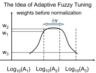
(either positive or negative) parameter𝐾𝑐can be set, to which a small positive parameter𝐴𝑐fits well. In the great majority of the applications a single parameter𝐴𝑐does well. However, if problems arise by leaving the bounded region of convergence a set of a few various 𝐴𝑐𝑖 parameters can also be used in (1) the obtain a set of possible next required values {𝑟(𝑖)𝑛+1}. The next required signal will be the weighted sum of these
“proposals” as𝑟𝑛+1=∑
𝑖∑𝑤𝑖
𝑗𝑤𝑗𝑟𝑛+1(𝑖) . In [19] simple scheme was proposed for obtaining the weights that is explained in Fig. 1. The weights are obtained by the use of a rigid, positive, bell-shaped function that is kept moving with fixed velocity over a grid: for decreasing response error ∣∣⃗ℎ𝑛∣∣ the direction of motion remains invariant, otherwise it is changed.
In this manner fine tuning of the adaptive controller was achieved. Though de details of the conditions of convergence
Fig. 1. Explanation of “fuzzy grid” used for fine tuning of the adap- tive control parameters{𝐴𝑐𝑖}first introduced in [19] and completed by rigidly shifting the whole grid in [20]
were detailed in [15] it worths noting that, as it can well be seen in (1), the properties of the partial differential ∂ ⃗𝑓(⃗𝑟∂⃗𝑟𝑛) certainly influence the convergence of the method since it𝑛
considerably influences the formation of the control sequences through ∂⃗𝑟∂⃗𝑟𝑛+1
𝑛 . Actually this quantity can be used for deciding if the choice 𝐵𝑐 = 1 or 𝐵𝑐 = −1 can be taken, as well as for deciding the proper range for ∣𝐾𝑐∣. In the particular examples considered instead of computing the components of the matrix ∂ ⃗𝑓(⃗𝑟∂⃗𝑟𝑛)
𝑛 the more easily computable scalar product [⃗𝑓(⃗𝑟𝑛)−⃗𝑓(⃗𝑟𝑛−1)][⃗𝑟𝑛−⃗𝑟𝑛−1]′ wasobserved for determining the controllability of the given stage of the process.
For developingobserversthe properties of the series given in (2) is utilized by the use of which forgetting filterscan be constructed for the discretetime-sequence of physical quanti- ties{𝑧(𝑡−𝑠)∣𝑠= 0, . . . ,∞}as¯𝑧(𝑡) = (1−𝛽)∑∞
𝑠=0𝛽𝑠𝑧(𝑡−𝑠) in which 𝑠 = 0 corresponds to the present instant, and the higher values pertain to the past (also used e.g. in [19]).
The old, rather “obsolete” information is forgotten faster for smaller 0 < 𝛽 < 1 values. For constant 𝑧(𝑖) ≡𝑧 evidently
¯
𝑧 = 𝑧 therefore (2) acts as a noise filter, too, that is able to average out fluctuations. From technical point of view the realization of this filter is very easy: a quantity 𝑧(𝑡)ˆ can be stored in a buffer and in each control cycle the refreshing operation𝑧(𝑡+1) :=ˆ 𝛽𝑧(𝑡)+𝑧(𝑡+1),ˆ 𝑧(𝑡) = (1−𝛽)ˆ¯ 𝑧(𝑡)can be applied. In the here presented simulations this method is used for the observation of chattering and that of the applicability of the adaptive control method.
Σ :=
∑∞ 𝑠=0
𝛽𝑠= 1
1−𝛽 <∞ if ∣𝛽∣<1 (2) During former investigations it was also observed that leaving the region of convergence not necessarily leads to the decay of the adaptive control. It trajectory tracking can remain precise at the cost of the appearance of big chattering in the control signal. In [20] simple method was successfully
suggested for the reduction of this chattering. According to that (1) can be modified as follows:
⃗ℎ𝑛+1:= ⃗𝑓(⃗𝑟𝑛)−⃗𝑟𝑑𝑛+1, ⃗𝑒𝑛+1:=⃗ℎ𝑛+1/∣∣⃗ℎ𝑛+1∣∣, 𝐵˜𝑛+1=𝐵𝑐𝜎(𝐴𝑐∣∣⃗ℎ𝑛+1∣∣),
⃗𝑟𝑛+1= (1 + ˜𝐵𝑛+1)⃗𝑟𝑛+𝐾𝑠𝜎(˜
𝐵𝑛+1𝐾𝑐
𝐾𝑠
)𝑂⃗𝑒𝑛+1. (3)
Besides that, by observing chattering the whole grid of pa- rameters {𝐴𝑐𝑖} can be shifted in Fig. 1 to the direction of the smaller values if chattering (i.e. strong fluctuation in the control signal) occurs. In Section III the particular physical systems are detailed for which the operation of the control method was investigated.
III. THE PARTICULARPARADIGMSUNDER
CONSIDERATION
In the investigations a Classical Mechanical system similar to that used in [18] wit the introduction of further asymmetries and “actual vs. reference system differences” within the frames of an MRAC controller. The other was the famousBrusselator Model of the Belousov-Zhabotinskii Reaction developed by Prigogine and Lefever in 1968 [21].
A. MRAC Control of Two Coupled Nonlinear Springs The dynamics of the actual and the reference systems are given by (4) and (5), respectively, with the parameter settings as 𝑚1 = 𝑚2 = 40𝑘𝑔, 𝑔 = 11𝑚/𝑠2 (gravitational acceleration), 𝐿1=𝐿2= 0.3𝑚,𝑘1=𝑘2= 260𝑁/𝑚3,𝑏1= 𝑏2= 1𝑁⋅𝑠/𝑚, and𝑚˜1= 10𝑘𝑔,𝑚˜2= 20𝑘𝑔,˜𝑔= 10𝑚/𝑠2, 𝐿˜1 = 0.9𝑚, 𝐿˜2 = 1.8𝑚, ˜𝑘1 = 160𝑁/𝑚4,˜𝑘2 = 380𝑁/𝑚4,
˜𝑏1 = 0.5𝑁 ⋅ 𝑠/𝑚,𝑏2 = 1𝑁 ⋅ 𝑠/𝑚. The kinematically prescribed PID-type tracking error relaxation was given as 𝑟𝑑(𝑡) := ¨𝑥𝐷𝑒𝑠(𝑡) = ¨𝑞𝑁𝑜𝑚(𝑡) + 3Λ[
˙
𝑞𝑁𝑜𝑚(𝑡)−𝑞(𝑡)˙ ] + 3Λ2[
𝑞𝑁𝑜𝑚(𝑡)−𝑞(𝑡)] +Λ3∫𝑡
0
[𝑞𝑁𝑜𝑚(𝜏)−𝑞(𝜏)]
𝑑𝜏 withΛ = 20/𝑠. For the two mass-points 3rd order spline functions were prescribed as nominal trajectories. The discrete time-resolution of the integration was 1𝑚𝑠.
𝑚1(¨𝑞1−𝑔) +𝑘1⋅( 𝑞1−𝐿˜1
)3
− 𝑘2⋅(𝑞2−𝑞1−𝐿2)3+𝑏1𝑞˙1=𝑄1
𝑚2(¨𝑞2−𝑔) +𝑘2⋅(𝑞2−𝑞1−𝐿2)3+𝑏2𝑞˙2=𝑄2 (4)
˜
𝑚1(¨𝑞1−𝑔) + ˜˜ 𝑘1⋅𝑠𝑖𝑔𝑛( 𝑞1−𝐿˜1
) (𝑞1−𝐿˜1
)4
−
˜𝑘2⋅𝑠𝑖𝑔𝑛(
𝑞2−𝑞1−𝐿˜2
)× (𝑞2−𝑞1−𝐿˜2
)4
+ ˜𝑏1𝑞˙1=𝑄1
˜
𝑚2(¨𝑞2−𝑔) + ˜˜ 𝑘2⋅𝑠𝑖𝑔𝑛(
𝑞2−𝑞1−𝐿˜2
)× (𝑞2−𝑞1−𝐿˜2
)4
+ ˜𝑏2𝑞˙2=𝑄2
(5)
The simulation results for the non-adaptive controller well reveal the consequences of the differences between the actual and the reference models in the trajectory tracking accuracy (Figs. 2, and 3). The adaptive control parameters were as follows: 𝐾𝑠 = 700𝑁, 𝐾𝑐 = 70000𝑁, 𝐵𝑐 = −1, initially
Fig. 2. Trajectory tracking of the non-adaptive controller for the coupled springs
Fig. 3. Tracking error of the non-adaptive controller for the coupled springs
𝐴𝑐 ∈ {10−3.55,10−3.50,10−3.45}, and 𝛽 = 0.5 in the forgetting buffer. The results of the adaptive controller for 𝑂 = 𝐼 (i.e. without any rotation for the direction of the response error) are given in Fig. 4, and 5. The tracking accuracy evidently became quite precise even in the case of the phase trajectories, too. The small chattering that is observable in the chart of the forces can well be revealed as well as the realization of the “MRAC illusion”:the desired forces calculated according to the reference model(green line for 𝑄1, red line for 𝑄2) are very close to that recalculated from the realized acceleration of the actual system and the reference model (brown line for 𝑄1, purple line for 𝑄2), andconsiderably differ from the actually exerted ones(black line for 𝑄1, blue line for 𝑄2). This difference corresponds to the adaptive deformation. Figure 6 testifies that though the tracking error increased for a 𝜑 = 0.8𝑟𝑎𝑑 rotation in the (𝑄1, 𝑄2) space the controller did not collapse and well maintained the MRAC illusion, too. (For sparing room the chart of the control forces is not shown now.)This definitely means a kind of robustness of the control method for Classical Mechanical systems.
Fig. 4. Tracking error of the adaptive controller for the coupled springs for𝑂=𝐼
Fig. 5. Forces of the adaptive controller for the coupled springs for 𝑂=𝐼
Fig. 6. Tracking error of the adaptive controller for the coupled springs for𝑂pertaining to0.8𝑟𝑎𝑑
B. RFPT-based Adaptive Control of the Brusselator Model The portmanteau “Brusselator” introduced by J.J. Tyson in 1976 in [22] refers to the Brussels School of Thermodynam- ics in which the first model of chemical oscillations were mathematically expounded. In [23] the reactions described by (6) were used with assumedly constant 𝐴 and𝐵 𝑚𝑜𝑙𝑒/𝐿 concentrations. In the present paper its modification (7) is applied with the assumption that in a stirred reactor vessel of volume 𝑉 𝐿 during a small time-interval 𝛿𝑡 𝑠 𝛿𝑁𝐴𝑚𝑜𝑙𝑒 ingress of the very dense reagent 𝐴 of negligible volume is introduced that does not observably dilute the other reagents in the vessel. Similar assumption was made for reagent 𝐵 that led to decoupled control signals as 𝑢𝐴 := 𝛿𝑁𝑉 𝛿𝑡𝐴 ≥0 and 𝑢𝐵 := 𝛿𝑁𝑉 𝛿𝑡𝐵 ≥ 0 of dimension 𝑚𝑜𝑙𝑒𝐿⋅𝑠 . Since the molecules 𝑋, 𝑌, 𝐷 and𝐸 are produced of 𝐴 and𝐵 in this approach replenishment of components 𝐴 and 𝐵 must be satisfactory for control purposes. Since the time-derivatives of the first two equations of (7) contained 𝐴˙ and 𝐵˙ a 2nd order PID- type control was designed for thedesired 𝑋¨𝑑 and𝑌¨𝑑 values (exactly of the same form that was considered in the case of the coupled springs) that so provided thedesired 𝐴˙𝑑 and𝐵˙𝑑 by the use of which𝑢𝐴and𝑢𝐵 were determined from the last two equations according to the available model.
In the forthcoming simulations the exact parameterswere assumed to be 𝑘1 = 1, 𝑘2 = 1, 𝑘3 = 1, and 𝑘4 = 1 while the approximate ones used by the controller were 𝑘˜1 = 0.8,
˜𝑘2 = 0.9, 𝑘˜3 = 0.7, and ˜𝑘4 = 0.6 of appropriate physical dimensions that comply with (7). The simulations made for Λ = 6/𝑠 for the non-adaptive simple PID controller for large amplitude (0.5𝑚𝑜𝑙𝑒𝐿 ) oscillation in the nominal trajectory of frequency 𝜔 = 3/𝑠 provided nice trajectory tracking but in it the physically not interpretable 𝑢𝐴 < 0, 𝑢𝐵 < 0, 𝐴 <0,𝐵 <0quantities also occurred. For getting rid of the physically not interpretable sessions (7) were completed with truncations for the negative values. This lead to completely unapplicable PID control that allowed fast rate of increase in certain concentrations with considerable positive ingress rates, however, since the extraction of pure reactants were impossible the decreasing phases were left without active control with long 𝑢𝐴 ≡ 0 and 𝑢𝐵 ≡ 0 sessions. These asymmetries are the main barriers of the available control speed. On this reason the fast transients of the iterative learning that were not critical in the case of the mechanical system were carefully avoided in the case of the chemical reaction by setting thecycle time of the controller10𝑚𝑠and the discrete time-resolution of the Euler integration to 1𝑚𝑠.
Furthermore nominal trajectory of considerably smaller am- plitude𝐻 = 0.05𝑚𝑜𝑙𝑒𝐿 was considered for which the common PID controller provided useful results (Fig. 7). The results obtained for the adaptive counterpart of the controller for the same nominal motion are given in Fig. 8 for the adaptive parameter settings 𝐾𝑐 = 600, 𝐾𝑠 = 5𝑚𝑜𝑙𝑒𝐿⋅𝑠2, 𝐵𝑐 = −1, and 𝐴𝑐 ∈ {1.67,5.27,16.67,52.70,166.67,527.05} ×10−5 𝑚𝑜𝑙𝑒𝐿⋅𝑠2. The adaptivity was switched on at 𝑡 = 5𝑠 when the rough initial transients were already damped by the common PID
Fig. 7. Tracking error of the simple non-adaptive PID controller in the non-transient stage (for 𝑋: black and green lines, for 𝑌: blue and red lines)
controller and further refinement of the tracking properties became actual. The improvement in the tracking precision in the stabilized stage of the motion is evident.
𝐴→𝑘1 𝑋, 𝐵+𝑋 →𝑘2 𝑌 +𝐷,
2𝑋+𝑌 →𝑘3 3𝑋, 𝑋 →𝑘4 𝐸. (6) 𝑋˙ =𝑘1𝐴−𝑘2𝐵𝑋+𝑘3𝑋2𝑌 −𝑘4𝑋,
𝑌˙ =𝑘2𝐵𝑋−𝑘3𝑋2𝑌, 𝐴˙=−𝑘1𝐴+𝑢𝐴,𝐵˙ =−𝑘2𝐵𝑋+𝑢𝐵.
(7) Figure 9 reveals the details of the adaptation mechanism.
IV. CONCLUSIONS
Very briefly it can be stated that the RFPT-based adaptive controllers can efficiently used either for mechanical and chemical systems. In the latter case especial emphasis must be placed on the phenomenological limitations of the system that manifest themselves mainly as speed limitations.
Regarding further research it seems to be expedient to make investigations for more realistic control signals that take into account the effect that the ingress of a certain component also dilutes the other ones in the reaction vessel. For fixing the volume of reaction certain outflow rate must also be allowed.
ACKNOWLEDGMENT
The authors gratefully acknowledge the support provided by the National Development Agencyand theHungarian Na- tional Scientific Research Fund (OTKA CNK 78168) as well as the grant provided by the project T ´AMOP-4.2.2/B-10/1- 2010-0020 (Support of the scientific training, workshops, and establish talent management system at the ´Obuda University).
REFERENCES
[1] A.M. Lyapunov,A general task about the stability of motion(in Russian), PhD Thesis, 1892.
[2] A.M. Lyapunov, Stability of motion, Academic Press, New-York and London, 1966.
[3] R. Isermann, K.H. Lachmann, and D. Matko,Adaptive Control Systems, New York DC, Prentice-Hall, USA, 1992.
Fig. 8. Tracking of the adaptive controller (for𝑋: black and green lines, for𝑌: blue and red lines)
[4] Jean-Jacques E. Slotine, W. Li,Applied Nonlinear Control, Prentice Hall International, Inc., Englewood Cliffs, New Jersey, 1991.
[5] R.M. Murray, Z. Li, S.S. Sastry,A mathematical introduction to robotic manipulation, CRC Press, New York, 1994.
[6] C.C. Nguyen, S.S. Antrazi, Zhen-Lei Zhou, C.E. Campbell Jr.,Adaptive control of a stewart platform-based manipulator, Journal of Robotic Systems, Volume 10, Number 5, 1993, pp. 657–687, 1993.
[7] J. Soml´o, B. Lantos, P.T. C´at,Advanced robot control, Akad´emiai Kiad´o, 2002.
[8] K. Hosseini–Suny, H. Momeni, and F. Janabi-Sharifi,Model Reference Adaptive Control Design for a Teleoperation System with Output Pre- diction, J Intell Robot Syst, DOI 10.1007/s10846-010-9400-4, pp. 1–21, 2010.
[9] C.J. Khoh and K.K. Tan,Adaptive robust control for servo manipulators, Neural Comput & Applic, vol. 12, pp. 178–184, 2005.
[10] Y. Li, K.C. Ng, D.J. Murray-Smith, G.J. Gray and K.C. Sharman, Genetic algorithm automated approach to design of sliding mode control systems,International Journal of Control, 1996, vol. 63, issue 4, pp 721- 739.
[11] I. Sekaj and V. Vesel´y, Robust Output Feedback Controller Design:
Genetic Algorithm Approach,IMA J Math Control Info, 2005, vol. 22, no. 3, pp 257-265.
[12] J.L. Chen, Wei-Der Chang, Feedback linearization control of a two- link robot using a multi-crossover genetic algorithm,Expert Systems with Applications, 2009, vol. 36, issue 2, part 2, pp 41544159.
[13] T.A. V´arkonyi, J.K. Tar, I.J. Rudas, Robust Fixed Point Transformations in Chaos Synchroniztion,Proc. of the 11th International Symposium of Hungarian Researchers on Computational Intelligence and Informatics, Budapest, November 18-20, 2010, pp. 219–224, 2010.
[14] J.K. Tar, L. N´adai, I.J. Rudas, T.A. V´arkonyi, Adaptive emission control of freeway traffic using quasi-stationary solutions of an approximate hydrodynamic model, Journal of Applied Nonlinear Dynamics, vol. 1 no. 1, pp. 29–50, April, 2012.
[15] J.K. Tar, J.F. Bit´o, L. N´adai, J.A. Tenreiro Machado, Robust Fixed Point
Fig. 9. The “desired” (𝑋¨: black, 𝑌¨: blue), adaptively deformed
“required”(𝑋¨: magenta,𝑌¨: purple), and therealized(𝑋¨: green,𝑌¨: red) signals of the adaptive controller, and the control signals (𝑢𝐴: black, 𝑢𝐵: blue)
Transformations in Adaptive Control Using Local Basin of Attraction, Acta Polytechnica Hungarica, Vol. 6 Issue No. 1, pp. 21–37, 2009.
[16] J.K. Tar, J.F. Bit´o, I.J. Rudas, Replacement of Lyapunov’s Direct Method in Model Reference Adaptive Control with Robust Fixed Point Transformations,Proc. of the 14th IEEE International Conference on Intelligent Engineering Systems 2010, Las Palmas of Gran Canaria, Spain, May 5–7, pp. 231–235, 2010.
[17] R.E. Kalman, A New Approach to Linear Filtering and Prediction Problems,Transactions of the ASMEJournal of Basic Engineering, Vol.
82 (Series D), pp. 35–45, 1960.
[18] J.K. Tar, I.J. Rudas, T.A. V´arkonyi, Simple Practical Methodology of Designing Novel MRAC Controllers for Nonlinear Plants,Proc. of the 2012 IEEE/ASME International Conference on Advanced Intelligent Mechatronics, July 11-14, Kaohsiung, Taiwan, pp. 928–933, 2012.
[19] J.K. Tar, L. N´adai, I.J. Rudas, T.A. V´arkonyi, RFPT-based Adaptive Control Stabilized by Fuzzy Parameter Tuning,Proc. of the 9th European Workshop on Advanced Control and Diagnosis, ACD 2011. Budapest, Hungary,pp. 1–8. Paper 6, 2011.
[20] T.A. V´arkonyi, J.K. Tar, I.J. Rudas, I. Kr´omer, VS-type Stabilization of MRAC Controllers Using Robust Fixed Point Transformations,Proc.
of the 7th IEEE International Symposium on Applied Computational Intelligence and Informatics, May 2426, 2012, Timis¸oara, Romania, pp.
389–394, 2012.
[21] I. Prigogine, R. Lefever, Symmetry Breaking Instabilities in Dissipative Systems II,J Chem Phys, Vol. 48, pp. 1695–1700, 1968.
[22] J.J. Tyson, The Belousov-Zhabotinskii Reaction, Lecture Notes in Biomathematics 10, Springer-Verlag, Heidelberg, 1976.
[23] D. Kondepudi and I. Prigogine,Modern Thermodynamics, John Wiley
& Sons, Chichester, 1998.