Adaptive Emission Control of Freeway Traffic via Compensation of Modeling Inconsistences

Adaptive Emission Control of Freeway Traffic via Compensation of Modeling Inconsistences

Ter´ez A. V´arkonyi^∗, J´ozsef K. Tar^†, Imre J. Rudas^†

∗Doctoral School of Applied Informatics, John von Neumann Faculty of Informatics Obuda University´

96/B B´ecsi street, Budapest, H-1034, Hungary varkonyi.teri@phd.uni-obuda.hu

†Institute of Intelligent Engineering Systems, John von Neumann Faculty of Informatics Obuda University´

96/B B´ecsi street, Budapest, H-1034, Hungary tar.jozsef@nik.uni-obuda.hu, rudas@nik.uni-obuda.hu

Abstract—Nowadays when traffic jams and air pullution are very common, controlling the emission rate of the exhaust fumes is a significant task. Many difficulties make this problem more sophisticated, for example the present emission models sometimes need too many information so it is quite complex to work with them. On the other hand, the underlaying physics behind the hydrodynamic traffic models does not suggest unique mathematical formulation so we need adaptive controllers that iteratively improve the forecasts obtained by a rough initial model without tuning the parameters of a particular mathematical structure. In this paper a simple method is shown for determining the stationary solutions obtained from a hydrodynamic model for a realistic parameter range. The method is based on Robust Fixed Point Transformations (RFPT)-based adaptive control that needs only the main factors in the emission: the traffic density and velocity. For controlling it applies electric road signs for the prescribed velocities and allowed ingress rate from the ramp in the preceding sector. This is a new area for the RFPT, but as the simulations show it is successfully applyable to the problem.

I. INTRODUCTION

The relationship between freeway traffic and health has been investigated for a long time, e.g. [1]. An important point of view is the emission rate of exhaust fumes, because under various meteorological conditions different emission rates can dissolve in the environment. The chemical composition of the exhaust depends on the actual traffic conditions (road slope, tyre friction, deceleration/acceleration and velocity), the particular properties of the various vehicles (engine types, their gearing system [2], etc.). For modeling these effects quite complex models were developed (e.g. [3], [4], [5], [6]) but their practical use is limited because normally the traffic control systems do not have enough information they need.

Development of proper models for the road traffic is also an interesting question. Certain investigations have revealed fractional order dynamics in the nature of freeway traffic [7]. Several models can be regarded as some mathematical approximations of continuum mechanical ones that use integer order partial derivatives (e.g. [8], [9], [10], [11], [12], [13], [14]) in which the time is kept as continuous variable but the

space is treated as a discretized grid. This discretization can be realized by the use of various numerical approximations of the gradient operator that lead to models of various complexity.

Either one-sided or centralized differences can be applied without deeper physical substantiation. Since the underlaying physics behind the hydrodynamic traffic models does not suggest unique mathematical formulation we need adaptive controllers that iteratively improve the forecasts obtained by a rough initial model without tuning the parameters of a particular mathematical structure.

For similar purposes various Model Reference Adaptive Controllers (MRAC) can be found in the literature applied in robotics (e.g. [15], [16], [17], [18]) that use Lyapunov’s

“direct” method (e.g. [19], [20]) which can be a difficult technique that requires good mathematical skills in some cases.

Alternative, also effective techniques generating convergent sequences by the use of contractive maps in iterative learning control were also published (e.g. [21], [22], [23], [24], which is called Robust Fixed Point Transformations (RFPT).

In this paper a new approach is shown for determining the stationary solutions of emission control obtained from a hydrodynamic model for a realistic parameter range. The method is based on RFPT that needs only the main factors in the emission: the traffic density and velocity. For controlling it applies electric road signs for the prescribed velocities and allowed ingress rate from the ramp in the preceding sector.

The method is less complex compared to the ones mentioned above. This is a new area for the RFPT, but as the simulations show it is successfully applyable to the problem.

The paper is organized as follows: the hydrodynamic models of freeway traffic are presented in Section II. The stationary solutions of the dynamic model under the particular boundary conditions applied are shown in III. The simulation results are detailed ins Section IV. Section V contains the discussion of the results and proposes further researches in this direction.

II. HYDRODYNAMIC MODELS OF FREEWAY TRAFFIC

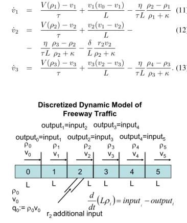
For our investigations, we use the model shown in Fig [?].

For simplicity let’s assume a one dimensional state varible which has six segments, from 0 to 5. The road segments have equal lengths L. Segments 0 and 5 represent the boundary conditions determining the propagation of thestate variables of segments 1 to 4 by keeping time as continuous variable, and applies discretized approximation of the –in this case one dimensional– space variable. The state variables are the vehicle density ρ (i.e. the number of vehicles over road segments of unit length), and the velocity of traffic v of a compressible fluid model. The quantity ρv (1/s) denotes the traffic current densityby the use of whichconservation of the vehiclescan be described by Eqs (2)-(5).

˙ v_i= ∂v_i

∂t +

3

X

s=1

∂v_i

∂xs

˙ x_s= v_i

∂t+

3

X

s=1

∂v_i

∂xs

v_s(x, t) (1)

˙

ρ₁ = q₀−ρ₁v₁

Lλ (2)

˙

ρ2 = ρ1v1−ρ2v2+r2

Lλ (3)

˙

ρ3 = ρ₂v₂−ρ₃v₃

Lλ (4)

˙

ρ₄ = ρ3v3−ρ4v4

Lλ (5)

˙

v₂ = V(ρ2)−v2

τ +v2(v1−v3)

2L − (6)

− η τ2L

ρ₃−ρ₁ ρ2+κ − δ

L r₂v₂ ρ2+κ

˙

v₁ = V(ρ₁)−v₁

τ +v₁(v₀−v₂)

2L − η

τ2L

ρ₂−ρ₀ ρ1+κ (7)

˙

v₃ = V(ρ₃)−v₃

τ +v₃(v₂−v₄)

2L − η

τ2L

ρ₄−ρ₂ ρ3+κ (8)

˙

v₄ = V(ρ₄)−v₄

τ +v₄(v₃−v₅)

2L − η

τ2L

ρ₅−ρ₃ ρ4+κ (9) According to Fig. 1 these equations apply the finest avail- able spatial resolution and they can be regarded as an integral form in the Gauss Equation that relates the time derivative of the number of vehicles within a fixed road segment with the ingress and egress of traffic flow at the boundaries of this segment. Thedynamic behaviorof this system is described by Eqs (7)-(9) in which for the V(ρ) functions various sugges- tions can be found in the literature as e.g. the Greenshields and thePapageorgiou models(10).

V(ρ) :=vf ree

1−_2ρ^ρ

cr

or V(ρ) :=v_{f ree}exp

−¹_bh

ρ ρ_cr

ib (10)

in which the first relationship established by Greenshields may provide even negative velocities that are not allowed under normal conditions in a real traffic, while the second one, the Papageorgiou model always results in interpretable

nonnegative values. On this reason in the present paper we use this latter approach.

It worths noting that Eqs. (7)-(9) cannot unambiguously derived from the fluid mechanical model. For instance, in case of a 3D traffic model (that definitely has sense for aircrafts and submarines), be the use of the 3D tensor components of the velocity field of motion, vi(x, t) the acceleration along a flowpath in (1) contains the gradient of this field that is approximated by central differences in (7)-(9).

However, we also could use one-sided differences for the approximation of the gradient _∂x^∂vi

s as e.g. in the following equations. The complexity of the model using central differ- ences evidently exceeds that of the one-sided models.

˙

v₁ = V(ρ₁)−v₁

τ +v₁(v₀−v₁)

L − η

τ L ρ₂−ρ₁

ρ1+κ (11)

˙

v₂ = V(ρ₂)−v₂

τ +v₂(v₁−v₂)

L − (12)

− η τ L

ρ₃−ρ₂ ρ2+κ − δ

L r₂v₂ ρ2+κ

˙

v₃ = V(ρ₃)−v₃

τ +v₃(v₂−v₃)

L − η

τ L ρ₄−ρ₃

ρ3+κ.(13)

0 1 2 3 4 5

ρ₀ v₀ q₀:= ρ₀v₀

ρ₁ v₁ ρ₀

v₀

ρ₂ v₂

ρ₃ v₃

ρ₄ v₄

ρ₅ v₅

r₂ additional input

L L L L L L

Discretized Dynamic Model of Freeway Traffic

output₀=input₁

output₁=input₂

output₂=input₃

output₃=input₄

output₄=input₅

(

)

d

i −

ρ

Fig. 1. The discretized hydrodynamic model of freeway traffic.

If the additional ingress rate from the ramp r2 is applied at section 2 and we apply central differences the appropriate dynamic model is given by Eqs (2)-(9). If we use electronically controlled road signs the quantitiesρ₀,v₀(consequentlyq₀:=

ρ₀v₀),v₄ andv₅ can be set as constant boundary conditions which together with Eq (9) withv˙₄= 0immediately determine the density in segment 5, ρ₅. Therefore the state variables remain only ρ₁,ρ₂,ρ₃,ρ₄,v₁,v₂, and v₃ for which we have coupled first order nonlinear differential equations.

We note that these equations describe a strongly “underac- tuated” system: we have only one time-varying control signal r₂ that influences the propagation of seven state variables.

Therefore we can precisely control only one of these variables or a well defined complex expression calculated from them,

or we can apply a kind of optimal controller in which a goal or cost function may describe weighted significance of the precision of controlling the individual variables so resolving the essentially contradiction-burdened task.

III. THE IDEA OF THE ADAPTIVE CONTROLLER USING QUASI-STATIONARY APPROACH

Further significant observation concerns thestability of the stationary solutions of these differential equations. Assume that for fixed rˆ2 stationary solutions (i.e. ρˆ1, ρˆ2,ρˆ3, ρˆ4, ˆv1, ˆ

v2, andvˆ3) for which˙ˆρ1= 0,˙ˆρ2= 0,˙ˆρ3= 0,˙ˆρ4= 0,˙ˆv1= 0,

˙ˆv₂ = 0, and˙ˆv₃ = 0, but these solutions are unstable. Such a dynamic system could require very fast feedback signal in r₂ to stabilize the stationary solutions that would be a very difficult, but its practical implementation would be dubious.

But if the stationary solutions are stable, the control task can be approached in a far simpler and far more easily implementable manner. In this case small steps in the control signal can result in small modifications of the controlled quantities that automatically set themselves following a shorter or longer transient session. In this case the need for really dynamic control ceases. The system model can simply be used for determining the necessary small steps in r2 and instead of fast dynamic feedback a simple iterative controller can be designed for the compensation of the modeling errors. This approach is traditional e.g. in Thermodynamics and Chemistry when the states of the thermal equilibrium are stable or at least metastable, i.e. they show stability at least against small perturbations. The quasi-stationary thermodynamic processes model the sate propagation as a sequence of stationary states (e.g. [26], [27]. The stationary solutions of certain multiple- compartment process models of the human glucose-insulin system (e.g. [29], [28]) also show stability that eases their control. In the next section the stationary solution of our model under the given boundary conditions are investigated.

A. The stationary solutions of the dynamic model

Under the boundary conditions ρˆ0 =const., vˆ0 =const.

(consequently qˆ0 := ˆρ0vˆ0=const.), vˆ4 = const. and ˆv5 = const. for constant control signal ˆr2 = const. the dynamic equations take the form of

0 = qˆ₀−ρˆ₁ˆv₁

Lλ (14)

0 = ρˆ₁vˆ₁−ρˆ₂ˆv₂+ ˆr₂

Lλ (15)

0 = ρˆ2vˆ2−ρˆ3ˆv3

Lλ (16)

0 = ρˆ3vˆ3−ρˆ4ˆv4

Lλ (17)

0 = V( ˆρ1)−ˆv1

τ +ˆv1(ˆv0−ˆv2)

2L − η

τ2L ˆ ρ2−ρˆ0

ˆ

ρ₁+κ (18) 0 = V( ˆρ2)−ˆv2

τ +ˆv2(ˆv1−ˆv3)

2L − η

τ2L ˆ ρ3−ρˆ1

ˆ

ρ₂+κ (19)

− δ L

ˆ r2ˆv2

ˆ ρ₂+κ

0 = V( ˆρ3)−vˆ3

τ +vˆ3(ˆv2−vˆ4)

2L − η

τ2L ˆ ρ4−ρˆ2

ˆ

ρ₃+κ (20) with the explicit equation for ρˆ5 as

ˆ

ρ₅= ˆρ₃−^{τ2L( ˆρ}_η^4+κ)×h_{V( ˆρ}

4)−ˆv₄

τ +^ˆv4(ˆv_2L^3−ˆv5)i

. (21) Due to nonlinearities in Eqs (14)-(20) the stationary solu- tions can be found by some numerical technique. Our solution is detailed in the next subsection.

B. Determination of the stationary solutions

For reducing complexity, we use a simple method. The occurrence of( ˆρi+κ)in the denominators may cause division by zero in numerical algorithms, so in the 1st step such divisions were eliminated via multiplication in Eqs 14-20 resulting the equations

0 =f₄ := qˆ₀−ρˆ₁vˆ₁ (22) 0 =f5 := ρˆ1ˆv1−ρˆ2vˆ2+ ˆr2 (23) 0 =f₆ := ρˆ₂ˆv₂−ρˆ₃vˆ₃ (24) 0 =f7 := ρˆ3ˆv3−ρˆ4vˆ4 (25) 0 =f1 := 2L( ˆρ1κ)[V( ˆρ1)−vˆ1] + (26)

+ τ( ˆρ1+κ)ˆv1(ˆv0−vˆ2)−η( ˆρ2−ρˆ0) 0 =f2 := 2L( ˆρ2+κ)[V( ˆρ2)−vˆ2] + (27)

+ τ( ˆρ₂+κ)ˆv₂(ˆv₁−vˆ₃)−η( ˆρ₃−ρˆ₁)−

− 2τ δˆr2ˆv2

0 =f₃ := 2L( ˆρ₃+κ)[V( ˆρ₃)−vˆ₃] + (28) + τ( ˆρ3+κ)ˆv3(ˆv2−vˆ4)−η( ˆρ4−ρˆ2).

A formal possibility is to consider Eqs (22)-(28) as subjects of some optimization task. According to the classification of the optimization tasks published in [30] our task corresponds to the most general case in which both the goal function as well as the possible constraints are nonlinear. However, the number of the independent variables is not too big. With the help of MS Excel’s Solver it can be proved that there is dependence of the coefficients of therˆ2-based polynomial on

ˆ q0.

In the next section the main exhaust fume emission factors are briefly considered.

C. Introduction of the Emission Factor

For calculating the main factors (the emission rates), it is assumed that at high velocities in the freeway the most signif- icant dissipative factor is thedrag forcegenerated by eddying air that is proportional to the square of the velocity:F =Cv² in which theC coefficient depends on the particular vehicles.

At velocity v the power consumption of this drag force is F v = Cv³ which roughly determines its fuel consumption.

On a road segment of lengthLand vehicle densityρin a given moment Lρ vehicles produces LCρv³ power consumption which roughly determines the emission rate of exhaust fume

on this segment (C denotes some “average” for the various vehicles present on the segment). It is evident that it is very difficult to obtain information on C, however, the emission for any car still strongly depends on the factor Ef := ρv³ that easily and quickly can be measured by cheap and simple inductive loop detectors (e.g. [31], [32]). On this reason we refer to this quantity as the “emission factor” which in the case of stationary flow in segment 3 can also be expressed as E_f = (ˆq₀+ ˆr₂)v²₃ sinceρˆ₃ˆv₃= ˆq₀+ ˆr₂. Independently of the actual (unknown) value ofC this factor must be decreased if the contamination of air is too high, or it can be increased if the actual concentration of the exhaust in the air is under some prescribed threshold. On this reason we made direct polynomial fitting forEf, too.

To sum up the stationary behavior of the system in the given parameter range can well be approximated by a few simple matrices containing the coefficients of the polynomial fitting.

Simultaneous measurement ofρˆ3andvˆ3guarantees not having drastic estimation errors.

The last question is the stability of the stationary states.

Since the suggested method needs continuous observations in general it cannot promise “asymptotic stability” due to the principle of causality (any correction is possible only after the observation), but as the investigations revealed, it can guarantee stability.

IV. SIMULATION RESULTS

For the adaptive control of the emission factor at road segment 3 the 3rd order polynomial fitting of Ef is directly calculated. Utilizing the fact that it is found to be monotone increasing function ofrˆ₂ for arbitrary positiveqˆ₀investigated a simple function is written in SCILAB to find a model- based ˆr₂^Des value for a prescribed nominal Eˆ_f^{N om} ≡ Eˆ_f^Des emission factor. Thenon-adaptive controller immediately in- troduced this value to its available system model. Theadaptive controller introduced this corrected value into function G of equation ([24], [25]) to calculate the deformed “Required”

input into the rough system model. In the simulations the realisticδtsampling = 0.028h≈100.8svalue is chosen. The control parameters areKctrl=−1e10,Actrl= 5e−12, and Bctrl = 1. The allowed maximum discrete time step on the integrator was set toδtsampling/50.

Simulation were made for the exact and the approximate models. The approximate model parameters were set as fol- lows: the values marked by the tilde symbol (˜) represent the exact model values, and the original parameter set now corresponds to the rough approximation of the real data:

˜

v_{f ree}= 1.20v_{f ree},˜b= 1.2b,L˜ =L,ρ˜_cr= 1.2ρ_cr,τ˜= 1.2τ,

˜

η = 1.2η,κ˜ = 1.2κ,δ˜= 1.2δ, and ˜λ=λ. The trivially not available parameters’ values were overestimated by 20%.

In the first set the applicability of the polynomially fitted exact model was checked for use in a common non-adaptive controller. In the simulations qˆ₀ was varied in drastic steps while E_f^{N om} varied continuously. Figure 2 reveals that the fitted stationary approximation is in harmony with the output of the dynamic model. It can be observed that the sign of the

6 5 1.10e+007

1.15e+007

4 3 2 1 0 1.20e+007 1.25e+007 1.30e+007

1.05e+007

Tracking of E.F. vs. Time

6 1

0 1.0e+006 6.0e+005

5 4 3 2.0e+005

-2.0e+005

2

Tracking Error vs. Time

6 1

0 500 450

5 4 3 400

350 300

2

q0 vs. Time

Fig. 2. Emission factor tracking of thenon-adaptive controller using the exact model parametersof the controlled system:E_f^{N om}vs.Ef, inkm²/h³units

6 5 1.15e+007

1.20e+007

4 3 2 1 0 1.25e+007 1.30e+007

1.10e+007

Tracking of E.F. vs. Time

6 1

0 2.0e+006 1.5e+006

5 4 3 1.0e+006

5.0e+005 0.0e+000 -5.0e+005 -1.0e+006

2

Tracking Error vs. Time

6 1

0 550 500

5 4 3 450

400 350 300 250

2

q0 vs. Time

Fig. 3. Emission factor tracking of theadaptive controller using the exact model parametersof the controlled system:E^{N om}_f vs.Ef, inkm²/h³units.

tracking error in the great majority of the simulation time is identical, i.e. the approximation is a little bit biased.

In the next step it was investigated to what extent disturbs the adaptive controller the use of the exact model. Figure 4 well demonstrates that instead of the bias, the adaptive controller produces an error that fluctuates around zero.

In the next step the operation of the adaptive controller was investigated for the case in which the polynomially fitted stationary values originate from the approximate dynamic model. The results are given in Figs. 4.

In the above simulations can well be seen that the sharp jumps in qˆ0 generate jumps in the solutions. In the next investigations the variation of qˆ0 was made continuous and smooth. The non-adaptive controller works with a huge error that means that theEf very drastically depends on the model parameters that were modified to the tune of 20% only (Fig. 5).

The adaptive controller (results given in Fig. 6) yields precise tracking without sharp jumps.

6 5 1.4e+007

1.6e+007

4 3 2 1 0 1.8e+007 2.0e+007

1.2e+007

Tracking of E.F. vs. Time

6 1

0 2e+006 0e+000

5 4 3 -2e+006

-4e+006 -6e+006 -8e+006

2

Tracking Error vs. Time

6 1

0 550 500

5 4 3 450

400 350 300

2

q0 vs. Time

Fig. 4. Emission factor tracking of the adaptive controller using the approximate model parametersof the controlled system:E_f^{N om}vs.Ef, in km²/h³units.

6 5 2.0e+007

1.5e+007

4 3 2 1 0

Tracking of E.F. vs. Time

6 1

0 -7.50e+006 -8.00e+006

5 4 3 -8.50e+006

-9.00e+006 -9.50e+006 -1.00e+007 -1.05e+007

2

Tracking Error vs. Time

6 1

0 500 450

5 4 3 400

350 300

2

q0 vs. Time

Fig. 5. Emission factor tracking of thenon-adaptive controller using the approximate model parametersof the controlled system for smoothq0ingress rate:E^{N om}_f :-black,Ef:-blue lines inkm²/h³units, time is given inhunits.

In the above simulations the cycle time of the controller was very big (≈ 100s). In the practice in urban traffic the available time for crossing a street used to be about10s, so the best accuracy can be expected to this nice sampling time.

According to Fig. 7 really very nice tracking precision can be achieved.

V. CONCLUSIONS

In this paper a new adaptive emission controller is shown and compared to a nonadaptive one. Its simple structure ensures low complexity. The adaptive controller that is based on the simple 3rd order polynomial approach of the quasi- stationary states of a given model and the RFPT transfor- mations seems to be a prospective solution. It applies the ingress rate from the ramp in the preceding road segment as a control signal, and requires the measurement of the traffic velocity and vehicle density in the controlled segment. The

6 5 1.4e+007

1.6e+007

4 3 2 1 0 1.8e+007 2.0e+007

1.2e+007

Tracking of E.F. vs. Time

6 1

0 2e+006 0e+000

5 4 3 -2e+006

-4e+006 -6e+006 -8e+006

2

Tracking Error vs. Time

6 1

0 500 450

5 4 3 400

350 300

2

q0 vs. Time

6 5 120

125

4 3 2 1 0 130 135 140 145

115

The Velocities vs. Time

6 1

0 12 10

5 4 3 8

6 4 2

2

The densities vs. Time

6 1

0 700 600

5 4 3 500

400 300 200 100

0 2

r2 vs. Time

Fig. 6. Emission factor tracking of the adaptive controller using the approximate model parametersof the controlled system for smoothq0ingress rate:E^{N om}_f :-black,Ef:-blue lines inkm²/h³units in the upper chart;v1:- black,v2:-blue,v3:-green lines inkm/hunits,ρ1:-black,ρ2:-blue,ρ3:-green, ρ4:-red lines in1/kmunits in the lower chart, time is given inhunits.

adaptive controller applied iteratively learns by utilizing the recent value of the control signal and the recent observed behavior of the controlled system. The here applied “prelimi- nary” or experimental version must be completed with safety limitations that prevent negative ˆr2 at the ingress side that cannot be realized in an actual road. In similar manner, the occurrence of negative velocities has to be excluded on the same reason. From the theory of partial differential equations it is well known that the boundary conditions very significantly influence the behavior of the solutions. In the here considered example we applied a well defined boundary condition by prescribing constant ρ0,v0, andv4=v5 values. For practical applications fitted polynomial packages could be prepared for several reasonable ρ0, v0, and v4 = v5 combinations depending on some “typical” traffic situations.

ACKNOWLEDGMENT

This research was supported by theNational Development Agencyand theHungarian National Scientific Research Fund (OTKA CNK 78168).

6 5 1.4e+007

1.6e+007

4 3 2 1 0 1.8e+007 2.0e+007

1.2e+007

Tracking of E.F. vs. Time

6 1

0 0e+000 -2e+006

5 4 3 -4e+006

-6e+006 -8e+006

2

Tracking Error vs. Time

6 1

0 500 450

5 4 3 400

350 300

2

q0 vs. Time

6 5 125

130

4 3 2 1 0 135 140 145

120

The Velocities vs. Time

6 1

0 12 10

5 4 3 8

6 4 2

2

The densities vs. Time

6 1

0 800 700

5 4 3 600

500 400 300 200 100

0 2

r2 vs. Time

Fig. 7. Emission factor tracking of the adaptive controller using the approximate model parametersof the controlled system for smoothq0ingress rate and10scycle-time:E^{N om}_f :-black,Ef:-blue lines inkm²/h³ units in the upper chart;v1:-black,v2:-blue,v3:-green lines inkm/hunits,ρ1:-black, ρ2:-blue,ρ3:-green,ρ4:-red lines in1/kmunits in the lower chart, time is given inhunits.

REFERENCES

[1] World report on road traffic injury prevention, eds. Margie Peden, Richard Scurfield, David Sleet, Dinesh Mohan, Adnan A. Hyder, Eva Jarawan and Colin Mathers, World Health Organization, Geneva, 2004.

[2] C.-A. Dragos, S. Preitl, R.-E. Precup, D. Pirlea, C.-S. Nes, E.M. Petriu and C. Pozna: Modeling of a Vehicle with Continuously Variable Transmis- sion. Proc of the 19th International Workshop on Robotics in Alpe-Adria- Danube Region, Budapest, Hungary, June 23-25 (2010) pp. 441–446.

[3] Transportation Research Board - Highway Capacity Manual (2000).

[4] COST 346 Final Report, (2005)

[5] Emission factor modelling and database for light vehicles, Report nLTE 0523, June (2007).

[6] Emission factors from the model PHEM for the HBEFA Version 3, (2009).

[7] L. Figueiredo, J.A. Tenreiro Machado, and J.R. Ferreira: ”Dynamical Analysis of Freeway Traffic”, IEEE Transactions On Intelligent Trans- portation Systems, Vol. 5, No. 4, December 2004.

[8] P´eter, T., Bokor, J., Modeling road traffic networks for control. In: Prof the Hon Dr Stephen Martin (eds) Annual international conference on network technologies & communications (NTC 2010), Thailand, 30th november 2010, pp. 18-22, 2010.

[9] S.P. Hoogendoorn and P. H. L. Bovy: State-of-the-art of vehicular traffic flow modelling. Proceedings of the Institution of Mechanical Engineers, Part I: Journal of Systems and Control Engineering, 215(4):283-303, 2001.

[10] Turner-Fairbank: Traffic Flow Theory and Characteristics.

http://www.tfhrc.gov/its/tft/tft.htm

[11] T. Luspay et al: Parameter-dependent modeling of freeway traffic flow.

Trasportation Research Part C, 2009. doi:10.1016/j.trc.2009.09.005 [12] T. Tettamanti, I. Varga & T. P´eni: MPC in urban traffic management.

Model Predictive Control, edited by: Tao Zheng, Publisher: InTech, Pub- lishing date: August (2010).

[13] C. Diakaki, M. Papageorgiou, K. Abodoulas: A multivariable regulator approach to traffic-responsive network-wide signal control. Control Engi- neering Practice 10 (2002) 183195.

[14] M. Papageorgiou: Dynamic Traffic Flow Modeling and Control, Short Course Notes, (2010).

[15] C.C. Nguyen, S.S. Antrazi, Z.-L. Zhou, C.E. Campbell Jr.: Adaptive con- trol of a stewart platform-based manipulator, Journal of Robotic Systems, Volume 10, Number 5 (1993) pp. 657–687.

[16] R. Kamnik, D. Matko and T. Bajd: Application of Model Reference Adaptive Control to Industrial Robot Impedance Control, Journal of Intelligent and Robotic Systems, vol. 22 (1998) pp. 153–163.

[17] J. Soml´o, B. Lantos, P.T. C´at: Advanced robot control, Akad´emiai Kiad´o, Budapest, Hungary (2002).

[18] K. Hosseini-Suny, H. Momeni, and F. Janabi-Sharifi: Model Reference Adaptive Control Design for a Teleoperation System with Output Predic- tion, J Intell Robot Syst, DOI 10.1007/s10846-010-9400-4, pp. 1–21, 2010.

[19] A.M. Lyapunov: A general task about the stability of motion (in Russian), PhD Thesis, University of Kazan, Russia, 1892.

[20] A.M. Lyapunov: Stability of motion. Academic Press, New-York and London, 1966.

[21] J.K. Tar, J.F. Bit´o, I.J. Rudas, K.R. Kozłowski, J.A. Tenreiro Machado:

Possible Adaptive Control by Tangent Hyperbolic Fixed Point Transfor- mations Used for Controlling the Φ⁶-Type Van der Pol Oscillator, in theProc. of the 6th IEEE International Conference on Computational Cybernetics (ICCC 2008), November 27–29, 2008, Hotel Academia, Star Lesn, Slovakia, pp. 15–20.

[22] J.K. Tar, J.F. Bit´o, L. N´adai, J.A. Tenreiro Machado: Robust Fixed Point Transformations in Adaptive Control Using Local Basin of Attraction, Acta Polytechnica Hungarica, Vol. 6 Issue No. 1 (2009) pp. 21–37.

[23] I.J. Rudas, J.K. Tar, T.A. V´arkonyi: Novel Adaptive Synchronization of Different Chaotic Chua Circuits, in Proc. of the ETAI COSY 2011, Special International Conference on Complex Systems: Synergy, of Control, Com- munications and Computing, COSY 2011, 16-20 September 2011, Ohrid, Macedonia, pp. 109–114.

[24] J.K. Tar, J.F. Bit´o, I.J. Rudas: Replacement of Lyapunov’s Direct Method in Model Reference Adaptive Control with Robust Fixed Point Transformations, Proc. of the 14th IEEE International Conference on Intelligent Engineering Systems 2010, Las Palmas of Gran Canaria, Spain, May 5–7, pp. 231–235, 2010.

[25] J.K. Tar, J.F. Bit´o, I.J. Rudas, K. Eredics: Comparative Analysis of a Traditional and a Novel Approach to Model Reference Adaptive Control.

Proc. of the 11th International Symposium of Hungarian Researchers on Computational Intelligence and Informatics, Budapest, November 18-20, (2010) pp. 93–98

[26] H.B. Callen: Thermodynamics and an Introduction to Thermostatistics, 2nd Edition, John Wiley & Sons Inc., 1985;

[27] D. Kondepudi, I. Prigogine: Modern Thermodynamics, John Wiley &

Sons, Chichester, 1998;

[28] C. Dalla Man, R. Rizza, and C. Cobelli: Meal simulation model of the glucose-insulin system,IEEE Transactions in Biomedical Engineering, vol.

54, no. 10, pp. 1740–1749, 2007.

[29] L. Magni, D.M. Raimondo,, C. Dalla Man, G. De Nicolao, B. Kovatchev, C. Cobelli: Model predictive control of glucose concentration in type I diabetic patients: An in silico trial, Biomedical Signal Processing and Control, vol. 4, no. 4, pp. 338–346, 2009.

[30] M. Baudin¹, V. Couvert¹, S. Steer²: Optimization in SCILAB,¹Scilab Consortium,²INRIA Paris - Rocquencourt, July 2010, www.scilab.org.

[31] M. Papageorgiou, A. Kotsialos: Freeway Ramp Metering: An Overview.

2000 IEEE Intelligent Transportation Systems Conference Proceedings Dearborn (MI), USA, October1-3, (2000).

[32] Traffic Detector Handbook: Third EditionVolume I. Research, De- velopment, and Technology Turner-Fairbank Highway Research Center.

Publication No. FHWA-HRT-06-108 October (2006).