Comparison of Michaelis-Menten kinetics modeling alternatives in cancer chemotherapy modeling
Dániel András Drexler, Tamás Ferenci, Anna Lovrics, and Levente Kovács
Abstract— Model-based optimization and personalization of tumor therapies require tumor growth models that reliably describe the effect of the drug used during the therapy.
A key phenomenon in the drug effect mechanism is the pharmacodynamics of the drugs which limits the maximal effect of the drug. The pharmacodynamics can be modeled with Michaelis-Menten kinetics, that can be realized in the differential equations of the model as a Hill function or bilinear functions with one extra state variable if we consider the quasi steady-state approximation or use triplet motifs, respectively.
We use experimental data for a chemotherapeutic drug and carry out parametric identification of our tumor model with both Michealis-Menten kinetics models. The results show that the quasi steady-state approximation has better modeling power and less complexity.
I. INTRODUCTION
Tumor growth dynamics modeling under the effect of different drugs is a key issue if we want to create personal- ized, optimal tumor therapies. The tumor models potentially enable us to use control engineering and mathematical meth- ods to optimize the tumor treatment [1], [2], [3], [4], [5], [6], [7], [8], [9], [10], [11]. A good tumor model captures tumor dynamics and drug dynamics as well, with realistic considerations, such as the effect of the drug on the tumor growth dynamics has an upper limit, while keeping the model structure as simple as possible. Simple structure is desirable for model analysis, many model-based optimization and con- trol design techniques and also for parametric identification.
The most popular tumor growth model modeling angio- genic therapies is the Hahnfeldt model [12], which captures the tumor and blood vessel dynamics, but lacks the modeling of pharmacodynamics and dead tumor volume. Based on experiments, the tumor contains dead and living regions in the case of antiangiogenic therapy, and there is no washout of the dead cells [13]. Moreover, the experiments have also showed that the pharmacodynamics of the drug can not be neglected, since giving one large dose according to the protocol had the same effect as giving 1/180 of the dose each day for an 18 days treatment period. This implies that after a limit, increasing the dose of the drug does not result in linear increase in the effect of the drug, but it has a plateau. This phenomenon is captured by the pharmacodynamics, and is
D. A. Drexler, T. Ferenci and L. Kovács are with the Physiological Controls Research Center, Research, Innovation and Service Center of Óbuda University, Óbuda University, Hungary {drexler.daniel,tamas.ferenci,kovacs.levente}
@nik.uni-obuda.hu
A. Lovrics is with the Membrane Protein Research Group, In- stitute of Enzymology, Hungarian Academy of Sciences, Hungary lovrics.anna@ttk.mta.hu
crucial for designing tumor therapies. The Hahnfeldt model has been modified and extended by other authors several times, but they did not incorporate neither pharmacodynam- ics nor dead regions [14]. A model with pharmacodynamics, dead regions and vasculature dynamics has been published recently [15].
A second-order model capturing tumor growth dynamics without dead regions and pharmacodynamics has been pub- lished in [16], and has been used for controller design in [17], [8], [18], [19], [20], [3]. The model has been extended with pharmacodynamics, mixed-order pharmacokinetics and dead tumor volume dynamics in [21]. This model uses Michaelis- Menten kinetics to describe the pharmacodynamics and phar- macokinetics as it will be described in Section II. Initially, the model was created to describe antiangiogenic therapy, thus it does not describe the dead tumor cell washout. The washout process can be added to the model by a simple linear term as suggested in [22].
There are two common methods to build-in Michaelis- Menten kinetics into our model. The first approach, which was used in [21], is the approximation of the Michaelis- Menten kinetics which supposes that the substrate reaches equilibrium much faster than the product, and results in a velocity term that is described by a Hill function. Applica- tion of the approximation of the Michaelis-Menten kinetics results in a third-order tumor model described in Section II. Another popular way to describe the Michaelis-Menten kinetics is by using triplets, i.e., using the stoichiometric equation of the Michaelis-Menten equation and consider mass-action kinetics, which results in bilinear velocity terms and an extra state corresponding to the enzyme-substrate complex, thus increasing the order of the model by one. We discuss this model in Section II and call it the fourth-order model.
We use experimental data from the Membrane Protein Research Group of the Hungarian Academy of Sciences published in [23]. The experiments are carried out on nine mice, using a cytotoxic agent called pegylated liposomal dox- orubicin (PLD) dosaged according to a protocol described in [23]. In some cases the mice in the experiments became resistant of the chemotherapy, however, our model is not capable to model this effect yet. Thus, we chose the set of measurements where resistance did not seem to be present (except for one case from the chosen measurement set).
We use mixed-effect models to carry out parametric iden- tification for both model structures. The methods used for identification are described in Section III, while the results of the identification are provided in Section IV. We show
that the third-order model which uses the quasi steady- state approximation of the Michaelis-Menten kinetics has much better modeling power. We end the paper with the conclusions in Section V.
II. THE TUMOR GROWTH MODEL
We define the tumor growth model equations with the help of stoichiometric equations using formal reaction kinetics analogy [24]. For the third-order model, the fictive species are X1, X2 and X3 that are the species representing the proliferating tumor volume, the dead tumor volume, and the drug level, respectively. The corresponding state variablesx1, x2 and x3 are the time functions of the proliferating tumor volume, dead tumor volume and drug level, respectively. The stoichimetric equations defining the underlying physiological phenomena are
• X1−−→a 2 X1that defines that the tumor cells proliferate (divide) with a tumor growth rate a. The correspond- ing term in the differential equation using mass-action kinetics is x˙1=ax1;
• X1 −−→n X2 that defines the necrosis (death) of tumor cells with necrosis rate n, which is the tumor necrosis that is independent of the treatment. Using mass-action kinetics, this equation modifies the dynamics of the proliferating and dead tumor volumes with the terms
˙
x1=−nx1,x˙2=nx1;
• X2−−→w O that defines the washout of the dead tumor cells with washout rate w. Using mass-action kinetics, this reaction step has the ratewx2. This extension was not present in [21], we use this term to define dead tumor cell washout which is a relevant process during chemotherapy, with the dynamicsx˙2=−wx2.
• X3 −−→c O that defines that there is an outflow of the drug with a reaction rate coefficientc, i.e. the clearance of the drug. We use the approximation of the Michaelis- Menten kinetics in order to have a mixed-order model for the pharmacokinetics, so this equations results in the termx˙3=−cx3/(KB+x3), where the parameterKB
is the Michaelis-Menten constant of the drug;
• X1+ X3
−−→b X2 that defines the effect mechanism of the drug in a general way, i.e., if living tumor and drug meets, they turn into dead tumor. The effect of the drug is considered with the approximation of the Michaelis- Menten kinetics with Michaelis-Menten constantED50 resulting in the velocity termx1x3/(ED50+x3). This effect on the volumes is considered with reaction rate coefficient b. The effect of this equation on the dy- namics of the proliferating and dead tumor volumes is expressed by the terms x˙1 = −bx1x3/(ED50+x3) and x˙2=bx1x3/(ED50+x3). We use the termx˙3=
−bkx1x3/(ED50+x3) which expresses the effect of this mechanism on the drug level dynamics, where the rate coefficient bk has the dimension mg/(kg · mm3· day).
The combination of these terms give the differential equation of the system:
˙
x1 = (a−n)x1−b x1x3
ED50+x3 (1)
˙
x2 = nx1+b x1x3
ED50+x3 −wx2 (2)
˙
x3 = −c x3
KB+x3 −bκ x1x3
ED50+x3 +u, (3) wherex1is the time function of proliferating tumor volume in mm3, x2 is the time function of dead tumor volume in mm3,x3 is the time function of drug level in mg/kg and u is the input that is the time function of drug injection rate in mg/(kg·day).
The outputyof the system is the measured tumor volume in mm3 that is the sum of the proliferating (x1) and dead (x2) tumor volumes, i.e.
y=x1+x2. (4) The dynamics of the output is described by the differential equation
˙
y=ax1−wx2 (5) that is the sum of (1) and (2), thus the change of the measured tumor volume depends directly only on the tumor growth rate constant a, the dead tumor washout w and the actual volume of the proliferating tumor volume and the dead tumor volume.
In the third-order model, we have used the approximation of the Michaelis-Menten kinetics with quasi steady-state. The model of the drug effect mechanism could be more accurate if we used Michaelis-Menten kinetics by supposing that the living tumor cell is the substrate, the drug is the enzyme, and using the stoichiometric equations
X1+ X3−−bb−−1
−1 X4−−→b2 X2+ X3
where X4 is a new species, the tumor-drug complex. This equation can model that the effect of the drug is not imme- diate, but there is an intermediate phase when the drug binds to the tumor and exerts its effect. The resulting differential equations of the fourth-order model are
˙
x1 = (a−n)x1−b1x1x3+b−1x4 (6)
˙
x2 = nx1−wx2+b2x4 (7)
˙
x3 = −c x3
KB+x3 −b1x1x3+ (b−1+b2)x4+u(8)
˙
x4 = b1x1x3−(b−1+b2)x4, (9) wherex1is the time function of proliferating tumor volume in mm3, x2 is the time function of dead tumor volume in mm3,x3 is the time function of drug level in mg/kg,uis the input that is the time function of drug injection rate in mg/(kg·day)and x4 is the tumor-drug complex volume in mm3.
The outputyof the system is the measured tumor volume in mm3that is the sum of the proliferating (x1) and dead (x2) tumor volumes and the tumor-drug complex volume (x4), i.e.
y=x1+x2+x4. (10)
The dynamics of the output is described by the differential equation
˙
y=ax1−wx2 (11) that is the sum of (6), (7) and (9), thus the change of the measured tumor volume depends directly only on the tumor growth rate constant a, the dead tumor washout w and the actual volume of the proliferating tumor volume and the dead tumor volume. Thus, the output dynamics is described by the same equation as in the case of the third-order model.
III. PARAMETRIC IDENTIFICATION
The differential equation systems were first converted to a – nonlinear – model where the parameters were assumed to be random effects. This means that every subject has an own realization for each parameter which is assumed to be a random draw from a given (usually normal) distribution, so that the number of estimated parameters is always fixed – two for normal distribution: mean and standard deviation – irrespectively of the number of subjects [25]. The mean measures the overall – population – value, while standard deviation characterizes the between-subject variability. An advantage of this model is that it handles the within-subject correlations, therefore these models are widely used to describe repeated-measures data and are also universally applied in population pharmacokinetics [26], [27].
Independence of random effects was assumed. Parameters were estimated on log scale, which ensures the positivity of the parameters. For the third-order model (1)-(3), the initial values were set to lna = −0.5, lnb = −2, lnED50 =
−9.9,lnbk =−14, lnc=−2, lnn=−2,lnx1(0) =−4, lnKB =−0.5 and lnw =−1, while for the fourth-order model (6)-(9), the initial values were set to lna = −1.5, lnb1 = −1.5, lnb−1 = −2, lnb2 = −1.5, lnc = −1.5, lnn = −2, lnx1(0) = −4, lnKB = −1.5 and lnw =
−0.5. Initial value for the standard deviation of the random effect was set to 0.01 for all parameters. Error term was assumed to be additive, with an initial value of1.
Estimation was performed with Stochastic Approximation Expectation-Maximization (SAEM) method which is one of the modern methods to solve the likelihood equations arising from the above-described nonlinear mixed effects models [28], [29]. Calculations were carried out under R statistical program package version 3.5.2 [30] using the librarynlmixrversion 1.0.0-7 [31].
IV. RESULTS
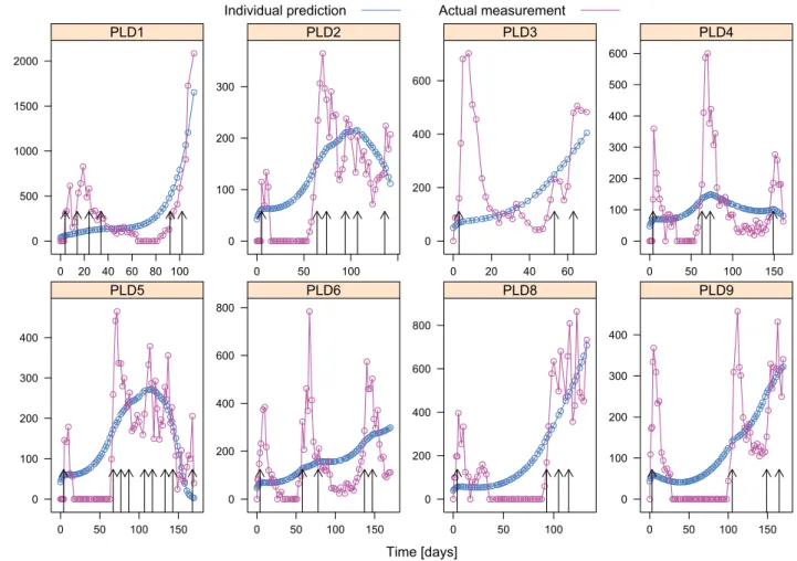
Figures 1 and 2 show the individual predicted tumor volume and the measurements for the third-order model and the fourth-order model, respectively. The vertical arrows indicate the days when the mice got injections, the dose was 8 mg/kg each time.
In the first case (PLD1 in the figures), the tumor acquires resistance during the therapy. This phenomenon is not in- corporated into the models, so the dynamics can not be described by neither of the models, and we got bad fits for both models. For cases 8 and 9 (PLD8 and PLD9), the measurements contain many zero values, however, in
reality the tumor volume was not zero, but it was too small for caliper measurements. These zero values complicate the identification process, and we get bad fits for these cases as well. For cases 2-6 (PLD2 - PLD6) we expect good fit results, since we can not observe acquired drug resistance and there are few zero measurements, so the models should be able to describe the dynamics governing the measured processes. Note that there is no case 7 (PLD7), since the measurements for that case in [23] were unavailable.
The third-order model shows good fit for cases 2-6 (Fig.
1), and can capture the individual dynamics for all these cases, even though it only uses an approximation of the Michaelis-Menten kinetics. Figure 2 shows that the fourth- order model could not capture the dynamics of the process, thus application of a more complex model is not desirable.
Although, the fourth-order model can capture the tendencies in the derivative, i.e., the increasing and decreasing segments in the trajectory, the amplitudes in the trajectory are not sufficient to describe the process.
Table I shows the estimation of the parameters for the fourth-order model. The parameterb1is only about one order of magnitude larger thanb−1, however, in the quasi steady- state approximation theb1parameter is supposed to be much larger than b−1 (i.e., with large order of magnitude). The value of these parameters may be responsible for the bad fit of the model. Note that since the identification problem is highly nonlinear, the result depends on the initial values used during the identification process.
V. CONCLUSIONS
The results showed that the third-order model can suffi- ciently describe the effect of chemotherapy on the tumor growth dynamics. The results have also showed that the fourth-order model is not able to describe the measurements.
This example has shown that increasing the model complex- ity does not increase the model capability of describing the measurements, on the contrary, it decreased the modeling power.
VI. ACKNOWLEDGMENTS
The authors would like to express their thanks to the Mem- brane Protein Research Group of the Hungarian Academy of Sciences for providing the measurement data. This project has received funding from the European Research Council (ERC) under the European Union’s Horizon 2020 research and innovation programme (grant agreement No 679681).
Anna Lovrics is supported by the Hungarian National Re- search, Development and Innovation Office (OTKA PD 124467). The research is partially supported by the Hungar- ian National Research, Development and Innovation Office (2018-2.1.11-TÉT-SI-2018-00007 and SNN 125739).
REFERENCES
[1] D. A. Drexler, L. Kovács, J. Sápi, I. Harmati, and Z. Benyó, “Model- based analysis and synthesis of tumor growth under angiogenic inhibition: a case study,”Proceedings of the 18th World Congress of the International Federation of Automatic Control, Milano, Italy, pp.
3753–3758, 2011.
Parameter Est. SE %RSE Back-transformed(95%CI) BSV(CV%) Shrink(SD)%
Log a -1.67 0.0364 2.18 0.188 (0.175, 0.202) 5.02% 32.9%>
Log b1 -1.78 0.0837 4.72 0.169 (0.144, 0.2) 9.23% 79.5%>
Log bm1 -2.32 0.0145 0.627 0.0986 (0.0959, 0.101) 2.13% 87.2%>
Log b2 -1.42 0.0824 5.8 0.242 (0.206, 0.284) 10.7% 56.7%>
Log c -1.48 0.141 9.53 0.228 (0.173, 0.301) 15.9% 72.2%>
Log n -1.9 0.039 2.05 0.149 (0.138, 0.161) 6.77% 19.6%<
Log x10 3.78 0.0645 1.71 44 (38.8, 49.9) 13.2% 36.5%>
Log KB -1.72 0.0194 1.13 0.179 (0.172, 0.186) 3.15% 80.0%>
Log w -0.591 0.232 39.2 0.554 (0.351, 0.872) 30.5% 68.6%>
149 149
TABLE I
ESTIMATED PARAMETERS OF THE NON-LINEAR MIXED EFFECTS MODEL(EST.), SE:STANDARD ERROR, RSE:RELATIVE STANDARD ERROR, CI:
CONFIDENCE INTERVAL, BSV:BETWEEN-SUBJECT VARIABILITY, CV:COEFFICIENT OF VARIATION, SD:STANDARD DEVIATION. LOG STANDS FOR NATURAL LOGARITHM.
Time [days]
Volume [mm3 ]
0 500 1000 1500 2000
0 20 40 60 80 100 PLD1
0 100 200 300
0 50 100
PLD2
0 200 400 600
0 20 40 60
PLD3
0 100 200 300 400 500 600
0 50 100 150
PLD4
0 100 200 300 400
0 50 100 150
PLD5
0 200 400 600 800
0 50 100 150
PLD6
0 200 400 600 800
0 50 100
PLD8
0 100 200 300 400
0 50 100 150
PLD9 Individual prediction Actual measurement
Fig. 1. Actual tumor volumes and (individual) estimations from the third-order model.
[2] H.-P. Ren, Y. Yang, M. S. Baptista, and C. Grebogi, “Tumour chemotherapy strategy based on impulse control theory,”Philosophical Transactions Mathematical Physical & Engineering Sciences, vol.
375, no. 2088, 2017.
[3] D. A. Drexler, J. Sápi, and L. Kovács, “H∞ control of nonlinear systems with positive input with application to antiangiogenic therapy,”
inProceedings of the 9th IFAC Symposium on Robust Control Design ROCOND 2018, 2018, pp. 146 – 151.
[4] D. A. Drexler, J. Sápi, A. Szeles, I. Harmati, A. Kovács, and L. Kovács,
“Flat control of tumor growth with angiogenic inhibition,”Proc. of the 7th International Symposium on Applied Computational Intelligence and Informatics, Timisora, Romania, pp. 179–183, 2012.
[5] L. Kovács, A. Szeles, J. Sápi, D. A. Drexler, I. Rudas, I. Harmati, and Z. Sápi, “Model-based angiogenic inhibition of tumor growth using modern robust control method,”Computer Methods and Programs in Biomedicine, vol. 114, pp. e98–e110, 2014.
[6] D. A. Drexler, J. Sápi, and L. Kovács, “Optimal discrete time control of antiangiogenic tumor therapy,”IFAC-PapersOnLine, vol. 50, no. 1, pp. 13 504 – 13 509, 2017, 20th IFAC World Congress.
[7] F. Cacace, V. Cusimano, A. Germani, P. Palumbo, and F. Papa, “Closed-loop control of tumor growth by means of anti-angiogenic administration,” Mathematical Biosciences &
Engineering, vol. 15, no. 4, pp. 827–839, 2018. [Online]. Available:
https://doi.org/10.3934/mbe.2018037
Time [days]
Volume [mm3 ]
0 500 1000 1500 2000
0 20 40 60 80 100 PLD1
0 100 200 300
0 50 100
PLD2
0 200 400 600
0 20 40 60
PLD3
0 100 200 300 400 500 600
0 50 100 150
PLD4
0 100 200 300 400
0 50 100 150
PLD5
0 200 400 600 800
0 50 100 150
PLD6
0 200 400 600 800
0 50 100
PLD8
0 100 200 300 400
0 50 100 150
PLD9 Individual prediction Actual measurement
Fig. 2. Actual tumor volumes and (individual) estimations from the fourth-order model.
[8] D. A. Drexler, J. Sápi, and L. Kovács, “Positive control of a minimal model of tumor growth with bevacizumab treatment,” inProceedings of the 12th IEEE Conference on Industrial Electronics and Applica- tions, 2017, pp. 2081–2084.
[9] J. Klamka, H. Maurer, and A. Swierniak, “Local controllability and optimal control for a model of combined anticancer therapy with control delays,”Mathematical Biosciences and Engineering, vol. 14, no. 1, pp. 195–216, 2017.
[10] D. A. Drexler, J. Sápi, and L. Kovács, “Positive nonlinear control of tumor growth using angiogenic inhibition,” IFAC-PapersOnLine, vol. 50, no. 1, pp. 15 068 – 15 073, 2017, 20th IFAC World Congress.
[11] F. S. Lobato, V. S. Machado, and V. Steffen, “Determination of an optimal control strategy for drug administration in tumor treatment using multi-objective optimization differential evolution,”Computer Methods and Programs in Biomedicine, vol. 131, pp. 51 – 61, 2016.
[12] P. Hahnfeldt, D. Panigrahy, J. Folkman, and L. Hlatky, “Tumor development under angiogenic signaling: A dynamical theory of tu- mor growth, treatment response, and postvascular dormancy,”Cancer Research, vol. 59, pp. 4770–4775, 1999.
[13] J. Sápi, L. Kovács, D. A. Drexler, P. Kocsis, D. Gajári, and Z. Sápi,
“Tumor volume estimation and quasi-continuous administration for most effective bevacizumab therapy,”PLoS ONE, vol. 10, no. 11, pp.
1–20, 2015.
[14] A. d’Onofrio and A. Gandolfi, “Tumor eradication by antiangiogenic therapy: analysis and extensions of the model by Hahnfeldt et al.
(1999),”Mathematical Biosciences, vol. 191, no. 2, pp. 159–184, 2004.
[15] D. Csercsik and L. Kovács, “Dynamic modeling of the angiogenic switch and its inhibition by bevacizumab,”Complexity, pp. 1–18, 2019.
[16] D. A. Drexler, J. Sápi, and L. Kovács, “A minimal model of tumor growth with angiogenic inhibition using bevacizumab,” inProceedings of the 2017 IEEE 15th International Symposium on Applied Machine
Intelligence and Informatics, 2017, pp. 185–190.
[17] G. Eigner and L. Kovács, “Linear matrix inequality based control of tumor growth,” in Proceedings of the 2017 IEEE International Conference on Systems, Man, and Cybernetics (SMC), 2017, pp. 1734–
1739.
[18] L. Kovács and G. Eigner, “Tensor product model transformation based parallel distributed control of tumor growth,”Acta Polytechnica Hungarica, vol. 15, no. 3, pp. 101–123, 2018.
[19] L. Kovács and Gy “A tp-lpv-lmi based control for tumor growth inhibition,” in Proceedings of the 2nd IFAC Workshop on Linear Parameter Varying Systems LPVS 2018, 2018, pp. 155 – 160.
[20] G. Eigner, D. A. Drexler, and L. Kovács, “Tumor growth control by tp-lpv-lmi based controller,” in Proceedings of the 2018 IEEE International Conference on Systems, Man, and Cybernetics (SMC), 2018, pp. 2564–2569.
[21] D. A. Drexler, J. Sápi, and L. Kovács, “Modeling of tumor growth incorporating the effects of necrosis and the effect of bevacizumab,”
Complexity, pp. 1–11, 2017.
[22] D. A. Drexler, I. Nagy, V. Romanovski, J. Tóth, and L. Kovács,
“Qualitative analysis of a closed-loop model of tumor growth con- trol,” in Proceedings of the 18th IEEE International Symposium on Computational Intelligence and Informatics, 2018, pp. 329–334.
[23] A. Füredi, K. Szebényi, S. Tóth, M. Cserepes, L. Hámori, V. Nagy, E. Karai, P. Vajdovich, T. Imre, P. Szabó, D. Szüts, J. Tóvári, and G. Szakács, “Pegylated liposomal formulation of doxorubicin overcomes drug resistance in a genetically engineered mouse model of breast cancer,”Journal of Controlled Release, vol. 261, pp. 287–296, 2017.
[24] P. Érdi and J. Tóth, Mathematical Models of Chemical Reactions.
Theory and Applications of Deterministic and Stochastic Models.
Princeton, New Jersey: Princeton University Press, 1989.
[25] J. Pinheiro and D. Bates, Mixed-effects models in S and S-PLUS.
Springer Science & Business Media, 2006.
[26] J. Owen and J. Fiedler-Kelly, Introduction to Population Pharma- cokinetic / Pharmacodynamic Analysis with Nonlinear Mixed Effects Models. Wiley, 2014.
[27] T. K. Kiang, C. M. Sherwin, M. G. Spigarelli, and M. H. Ensom,
“Fundamentals of population pharmacokinetic modelling,” Clinical pharmacokinetics, vol. 51, no. 8, pp. 515–525, 2012.
[28] B. Delyon, M. Lavielle, E. Moulines et al., “Convergence of a stochastic approximation version of the EM algorithm,”The Annals of Statistics, vol. 27, no. 1, pp. 94–128, 1999.
[29] W. Sukarnjanaset, T. Wattanavijitkul, and S. Jarurattanasirikul, “Eval- uation of FOCEI and SAEM estimation methods in population phar- macokinetic analysis using NONMEMR across rich, medium, and sparse sampling data,” European journal of drug metabolism and pharmacokinetics, vol. 43, no. 6, pp. 729–736, 2018.
[30] R Core Team, R: A Language and Environment for Statistical Computing, R Foundation for Statistical Computing, Vienna, Austria, 2018. [Online]. Available: https://www.R-project.org/
[31] M. Fidler, Y. Xiong, R. Schoemaker, J. Wilkins, M. Trame, T. Post, and W. Wang, nlmixr: Nonlinear Mixed Effects Models in Population Pharmacokinetics and Pharmacodynamics, 2018, r package version 1.0.0-7. [Online]. Available: https://CRAN.R- project.org/package=nlmixr