Modeling of tumor growth incorporating the effect of pegylated liposomal doxorubicin
Dániel András Drexler, Tamás Ferenci, Anna Lovrics, and Levente Kovács
Abstract— Modeling tumor growth is a fundamental step in the design of automated, optimal, patient specific therapies.
We extend our tumor growth model created to describe the effect of an angiogenic inhibitor in order to make it suitable to describe the effect of chemotherapy. By incorporating the dead tumor cell washout into our previous model, we are able to describe the most important phenomena during treatment with chemotherapy. We use measurements from experiments carried out on mice with a chemotherapeutic drug Pegylated Liposomal Doxorubicin, and carry out parametric identification of our model. The results show that the extended model can describe chemotherapy sufficiently.
I. INTRODUCTION
Modeling the tumor growth dynamics and the effect of dif- ferent drugs on tumor growth is a fundamental step towards personalized, optimized tumor therapies. The existence of a reliable tumor growth model lets us use control engineering and mathematical methods to optimize the tumor treatment [1], [2], [3], [4], [5], [6], [7], [8], [9], [10], [11]. A good tumor model captures tumor dynamics and drug dynamics as well, with realistic considerations such as the drug has a maximal effect of the tumor growth dynamics.
The most widely used tumor growth model in control applications is the Hahnfeldt model [12], which models the effect of angiogenic inhibitors, but lacks the modeling of pharmacodynamics and dead tumor volume. Experiments showed that in the case of antiangiogenic therapy, the tumor contains dead and living regions, and there is no washout of the dead cells [13]. Moreover, the experiments have also showed that the pharmacodynamics of the drug can not be neglected, since giving one large dose according to the protocol had the same effect as giving 1/180 of the dose each day for an 18 days treatment period. This shows that after a limit, increasing the dose of the drug does not result in linear increase in the effect of the drug, but it has a plateau. This phenomenon is captured by the pharmacodynamics, and is crucial for designing tumor therapies. The Hahnfeldt model has been modified and extended by other authors several times, but they did not incorporate neither pharmacodynam- ics nor dead regions [14]. A model with pharmacodynamics, dead tumor cell regions and vasculature dynamics has been published recently [15].
D. A. Drexler, T. Ferenci and L. Kovács are with the Physiological Controls Research Center, Research, Innovation and Service Center of Óbuda University, Óbuda University, Hungary {drexler.daniel,tamas.ferenci,kovacs.levente}
@nik.uni-obuda.hu
A. Lovrics is with the Membrane Protein Research Group, In- stitute of Enzymology, Hungarian Academy of Sciences, Hungary lovrics.anna@ttk.mta.hu
A minimalistic model capturing tumor growth dynamics without dead cell regions and pharmacodynamics has been published in [16], and has been used for controller design in [17], [8], [18], [19], [20], [3]. The model has been extended with pharmacodynamics, mixed-order pharmacokinetics and dead tumor volume dynamics in [21]. Although this model was validated with experimental results from antiangiogenic therapy, the model was formulated to be as general as possible. However, due to the nature of the measurements from antiangiogenic therapy [13], the model does not contain washout of the dead tumor cells, which is an important process in the case of chemotherapy [22]. We extend this model to incorporate dead tumor cell washout [23] and use the extended model to describe a therapy with a chemothera- peutic drug called Pegylated Liposomal Doxorubicin (PLD) [22].
We use experimental data from the Membrane Protein Research Group of the Hungarian Academy of Sciences published in [22]. We use the data acquired from experiments with PLD. In some cases the mice in the experiments became resistant of the chemotherapy, however, our model is not capable to model this effect yet. Thus, we chose the set of measurements where resistance did not seem to be present (except for one case from the chosen measurement set).
Our results show that the general model originally created for antiangiogenic therapy can sufficiently model the tumor growth dynamics even in the case of chemotherapy, as long as the tumors do not develop resistance against the drug.
The model extended with the dead tumor cell washout is discussed in Section II, while the methods used for parametric identification are detailed in Section III. The results of the identification are shown in Section IV, while the paper ends with the conclusions in Section V.
II. THE TUMOR GROWTH MODEL
We define the tumor growth model equations with the help of stoichiometric equations using formal reaction kinetics analogy [24]. The fictive species are the X1 proliferating tumor volume, the species X2 which represents the dead tumor volume, and the species X3 that represents the drug level. In the corresponding differential equations the state variables x1, x2 and x3 are the time functions of the proliferating tumor volume, dead tumor volume and drug level, respectively. The stoichiometric equations defining the underlying physiological phenomena are
• X1−−→a 2 X1that defines that the tumor cells proliferate (divide) with a tumor growth rate a. The correspond-
ing term in the differential equation using mass-action kinetics isx˙1=ax1;
• X1
−−→n X2 that defines the necrosis (death) of tumor cells with necrosis raten, which is the tumor necrosis that is independent of the treatment. Using mass-action kinetics, this equation modifies the dynamics of the proliferating and dead tumor volumes with the terms
˙
x1=−nx1,x˙2=nx1;
• X2 −−→w O that defines the washout of the dead tumor cells with washout ratew. Using mass-action kinetics, this reaction step has the ratewx2. This extension was not present in our original model [21].
• X3
−−→c O that defines that there is an outflow of the drug with a reaction rate coefficientc, i.e. the clearance of the drug. We use the approximation of the Michaelis- Menten kinetics in order to have a mixed-order model for the pharmacokinetics, so this equations results in the termx˙3=−cx3/(KB+x3), where the parameter KB
is the Michaelis-Menten constant of the drug;
• X1 + X3 −−→b2 X2 that defines the effect mechanism of the drug in a general way, i.e., if there is living tumor and drug, they turn into dead tumor. The ef- fect of the drug is considered with the approxima- tion of the Michaelis-Menten kinetics with Michaelis- Menten constant ED50 resulting in the velocity term x1x3/(ED50 + x3). This effect on the volumes is considered with reaction rate coefficientb. The effect of this equation on the dynamics of the proliferating and dead tumor volumes is expressed by the terms x˙1 =
−bx1x3/(ED50+x3)andx˙2=bx1x3/(ED50+x3).
The dimension of these velocity terms is mm3/day, thus these terms can not be directly used to modify the dynamics of the drug level, which has the dimension mg/(kg · day). Thus, we use the constant bk with dimension mg/(kg·mm3·day) to define the termx˙3=
−bkx1x3/(ED50+x3).
The combination of these terms give the differential equation of the system:
˙
x1 = (a−n)x1−b x1x3
ED50+x3
(1)
˙
x2 = nx1+b x1x3
ED50+x3 −wx2 (2)
˙
x3 = −c x3
KB+x3
−bk
x1x3
ED50+x3
+u, (3) wherex1 is the time function of proliferating tumor volume in mm3, x2 is the time function of dead tumor volume in mm3,x3 is the time function of drug level in mg/kg andu is the input that is the time function of drug injection rate in mg/(kg·day).
The outputyof the system is the measured tumor volume in mm3 that is the sum of the proliferating (x1) and dead (x2) tumor volumes, i.e.
y=x1+x2. (4) The dynamics of the output is described by the differential equation
˙
y=ax1−wx2 (5)
that is the sum of (1) and (2), thus the change of the measured tumor volume depends directly only on the tumor growth rate constanta, the necrotic washoutwand the actual volume of the proliferating tumor volume and the dead tumor volume.
III. PARAMETER ESTIMATION
The differential equation system was first converted to a – nonlinear – model where the parameters were assumed to be random effects. In brief, this means that every subject has an own value for each parameter which is assumed to be a random draw from a given (usually normal) distribution, hence the number of estimated parameters is always two – mean and standard deviation – regardless of the number of subjects [25]. The mean measures the overall – population – value, while standard deviation characterizes the between- subject variability. An advantage of this model is that it han- dles the within-subject correlations, therefore these models are widely used to describe repeated-measures data and are also universally applied in population pharmacokinetics [26], [27].
It was assumed that random effects are all independent from each other. All parameters were estimated on log-scale, which also ensures the positivity of the parameters. Initial values were set to lna = −0.5, lnb = −2, lnED50 =
−9.9, lnbk = −14, lnc = −2, lnn = −2, lnx1(0) =
−4, lnKB = −0.5 and lnw = −1. Initial value for the standard deviation of the random effect was set to0.01for all parameters. Error term was assumed to be additive, with an initial value of1. Estimation was performed with Stochastic Approximation Expectation-Maximization (SAEM) method which is one of the modern methods to solve the likelihood equations arising from the above-described nonlinear mixed effects models [28], [29]. Calculations were carried out under R statistical program package version 3.5.2 [30] using the librarynlmixrversion 1.0.0-7 [31].
IV. RESULTS
Table I shows the estimated mean (population) parameter values, along with their between-subject variability (mea- sured with coefficient of variation). The between-subject variability of parametersa,b,n,bk, andware less than 30 %.
However, the pharmacodynamics parameterED50 has large variability (152 %), thus the results show that the effective median dose changes greatly among mice. The initial tumor volume has the largest variability (6050%), however, this is not a model parameter, juts an initial value. Between subject variability is further illustrated in Figure 1 which uses dotplot to visualize the estimated (individual) value for each subject.
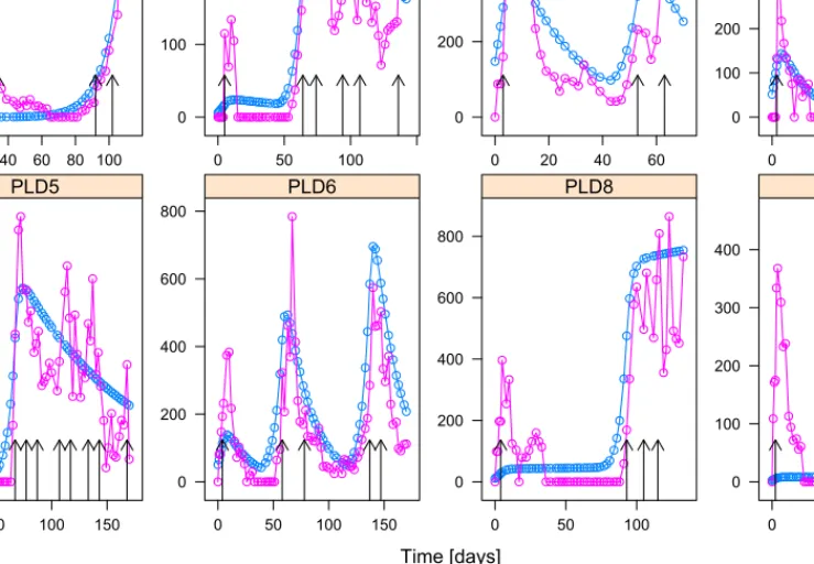
Results of the model, shown as the individual predicted tumor volume superimposed on the actual tumor volume are shown in Figure 2. The vertical arrows show the days when the mice got treatments. The dose was 8 mg/kg each time.
The model shows good individual fits for the cases 2-6.
For case 1 we can observe from the measurements that the tumor becomes resistant towards the drug during the therapy, which process is not incorporated into the model. The model neglects the initial phase when there is no resistance, and
Parameter Est. SE %RSE Back-transformed (95%CI) BSV (CV%) Shrink (SD)%
Loga -1.18 0.0744 6.28 0.306 (0.265, 0.354) 6.08% 33.2%>
Logb -1.79 0.14 7.8 0.166 (0.126, 0.219) 18.2% 11.8%<
Logc -1.36 0.126 9.29 0.257 (0.2, 0.329) 31.9% 10.4%<
Logn -1.94 0.0642 3.31 0.144 (0.127, 0.163) 16.3% 22.2%=
Logbk -14.3 0.0482 0.337 6.12e-007 (5.57e-007, 6.73e-007) 6.60% 85.0%>
Logx1(0) 1.94 0.802 41.4 6.94 (1.44, 33.4) 6050.% -1.74%>
LogKB -1.02 0.181 17.7 0.36 (0.253, 0.514) 34.5% 33.7%>
LogED50 -9.24 0.764 8.26 9.71e-005 (2.17e-005, 0.000434) 152.% 84.2%>
Logw -1.08 0.0783 7.26 0.34 (0.292, 0.397) 7.43% 81.6%>
Error 124 124
TABLE I
ESTIMATED PARAMETERS OF THE NON-LINEAR MIXED EFFECTS MODEL(EST.), SE:STANDARD ERROR, RSE:RELATIVE STANDARD ERROR, CI:
CONFIDENCE INTERVAL, BSV:BETWEEN-SUBJECT VARIABILITY, CV:COEFFICIENT OF VARIATION, SD:STANDARD DEVIATION. LOG STANDS FOR NATURAL LOGARITHM.
value
0.29 0.30 0.31 0.32 0.33
1 2
3 4 5
6
8 9
a
0.12 0.14 0.16 0.18 0.20
1
2 4 3
5 6 8 9
b
0.20 0.25 0.30 0.35
1 2
3 4
5
6 8
9
c
0.12 0.13 0.14 0.15 0.16 0.17
1 2
3 4
5 6
8 9
n
6.05e-07 6.10e-07 6.15e-07 1 2
3 4
5 6
8 9
bk
0 50 100 150
1
2 3
4 5
6 8
9
x10
0.25 0.30 0.35 0.40 0.45 0.50 1
2 3 4
5 6 8
9
KB
0.000080.000090.000100.000110.000120.00013 12
3
4 5
6
8 9
ED50
0.335 0.340 0.345
1 2
3 4
5 6
8 9
w
Fig. 1. Estimated individual parameters for each mouse.
learns the curve where the tumor became resistant towards the drug. By looking at Fig. 1, we can conclude that for case 1, the model has the largest tumor growth rate a and smallest necrotic raten and inhibition rate b, which results in ineffective therapy and uncontrollable tumor growth as it can be seen in Fig. 2. For cases 8 and 9, most of the parameters have average value compared to the other cases, except for the pharmacokinetic parameterscandKB, where theKB parameter is larger than for the other cases resulting
in faster depletion of the drug. As Fig. 2 shows, for cases 8 and 9 initially there is only one injection with a small effect according to the model, and according to the model the drug only had significant effect when the injections became frequent. Probably, in these cases the problem is not the resistance, but the nature of the measurements, since for most of the time the measured volume is assumed to be zero, but in reality there was some small tumor for both cases, but they were unmeasurable. Note that we do not have case 7,
since the measurement data was not accessible for the case indexed originally with 7 in [22].
V. CONCLUSIONS
The results showed that our general model is suitable for modeling the effect of chemotherapy as well after a mod- ification which incorporates dead tumor cell washout. The parametric identification showed that the pharmacodynamics parameterED50(the effective median dose of the drug) had the largest interpatient variability, while tumor growth rate a, necrotic washoutwand the rate of drug depletion due to the effectbk had the smallest interpatient variability. These results are important in therapy design, since the dosages must be aligned to the value of effective median dose.
The results showed that the model is not capable of describing the phenomenon when the tumor acquires drug resistance. However, this is not expected, since the model can not handle dynamics changes of the effect of the drug.
Incorporating this effect into the model is the subject of further research.
VI. ACKNOWLEDGMENTS
The authors would like to express their thanks to the Mem- brane Protein Research Group of the Hungarian Academy of Sciences for providing the measurement data. This project has received funding from the European Research Council (ERC) under the European Union’s Horizon 2020 research and innovation programme (grant agreement No 679681).
Anna Lovrics is supported by the Hungarian National Re- search, Development and Innovation Office (OTKA PD 124467). The research is partially supported by the Hungar- ian National Research, Development and Innovation Office (2018-2.1.11-TÉT-SI-2018-00007 and SNN 125739).
REFERENCES
[1] D. A. Drexler, L. Kovács, J. Sápi, I. Harmati, and Z. Benyó, “Model- based analysis and synthesis of tumor growth under angiogenic inhibition: a case study,”Proceedings of the 18th World Congress of the International Federation of Automatic Control, Milano, Italy, pp.
3753–3758, 2011.
[2] H.-P. Ren, Y. Yang, M. S. Baptista, and C. Grebogi, “Tumour chemotherapy strategy based on impulse control theory,”Philosophical Transactions Mathematical Physical & Engineering Sciences, vol.
375, no. 2088, 2017.
[3] D. A. Drexler, J. Sápi, and L. Kovács, “H∞ control of nonlinear systems with positive input with application to antiangiogenic therapy,”
inProceedings of the 9th IFAC Symposium on Robust Control Design ROCOND 2018, 2018, pp. 146 – 151.
[4] D. A. Drexler, J. Sápi, A. Szeles, I. Harmati, A. Kovács, and L. Kovács,
“Flat control of tumor growth with angiogenic inhibition,”Proc. of the 7th International Symposium on Applied Computational Intelligence and Informatics, Timisora, Romania, pp. 179–183, 2012.
[5] L. Kovács, A. Szeles, J. Sápi, D. A. Drexler, I. Rudas, I. Harmati, and Z. Sápi, “Model-based angiogenic inhibition of tumor growth using modern robust control method,”Computer Methods and Programs in Biomedicine, vol. 114, pp. e98–e110, 2014.
[6] D. A. Drexler, J. Sápi, and L. Kovács, “Optimal discrete time control of antiangiogenic tumor therapy,”IFAC-PapersOnLine, vol. 50, no. 1, pp. 13 504 – 13 509, 2017, 20th IFAC World Congress.
[7] F. Cacace, V. Cusimano, A. Germani, P. Palumbo, and F. Papa, “Closed-loop control of tumor growth by means of anti-angiogenic administration,” Mathematical Biosciences &
Engineering, vol. 15, no. 4, pp. 827–839, 2018. [Online]. Available:
https://doi.org/10.3934/mbe.2018037
[8] D. A. Drexler, J. Sápi, and L. Kovács, “Positive control of a minimal model of tumor growth with bevacizumab treatment,” inProceedings of the 12th IEEE Conference on Industrial Electronics and Applica- tions, 2017, pp. 2081–2084.
[9] J. Klamka, H. Maurer, and A. Swierniak, “Local controllability and optimal control for a model of combined anticancer therapy with control delays,”Mathematical Biosciences and Engineering, vol. 14, no. 1, pp. 195–216, 2017.
[10] D. A. Drexler, J. Sápi, and L. Kovács, “Positive nonlinear control of tumor growth using angiogenic inhibition,”IFAC-PapersOnLine, vol. 50, no. 1, pp. 15 068 – 15 073, 2017, 20th IFAC World Congress.
[11] F. S. Lobato, V. S. Machado, and V. Steffen, “Determination of an optimal control strategy for drug administration in tumor treatment using multi-objective optimization differential evolution,” Computer Methods and Programs in Biomedicine, vol. 131, pp. 51 – 61, 2016.
[12] P. Hahnfeldt, D. Panigrahy, J. Folkman, and L. Hlatky, “Tumor development under angiogenic signaling: A dynamical theory of tu- mor growth, treatment response, and postvascular dormancy,”Cancer Research, vol. 59, pp. 4770–4775, 1999.
[13] J. Sápi, L. Kovács, D. A. Drexler, P. Kocsis, D. Gajári, and Z. Sápi,
“Tumor volume estimation and quasi-continuous administration for most effective bevacizumab therapy,”PLoS ONE, vol. 10, no. 11, pp.
1–20, 2015.
[14] A. d’Onofrio and A. Gandolfi, “Tumor eradication by antiangiogenic therapy: analysis and extensions of the model by Hahnfeldt et al.
(1999),”Mathematical Biosciences, vol. 191, no. 2, pp. 159–184, 2004.
[15] D. Csercsik and L. Kovács, “Dynamic modeling of the angiogenic switch and its inhibition by bevacizumab,”Complexity, pp. 1–18, 2019.
[16] D. A. Drexler, J. Sápi, and L. Kovács, “A minimal model of tumor growth with angiogenic inhibition using bevacizumab,” inProceedings of the 2017 IEEE 15th International Symposium on Applied Machine Intelligence and Informatics, 2017, pp. 185–190.
[17] G. Eigner and L. Kovács, “Linear matrix inequality based control of tumor growth,” in Proceedings of the 2017 IEEE International Conference on Systems, Man, and Cybernetics (SMC), 2017, pp. 1734–
1739.
[18] L. Kovács and G. Eigner, “Tensor product model transformation based parallel distributed control of tumor growth,”Acta Polytechnica Hungarica, vol. 15, no. 3, pp. 101–123, 2018.
[19] L. Kovács and Gy “A tp-lpv-lmi based control for tumor growth inhibition,” in Proceedings of the 2nd IFAC Workshop on Linear Parameter Varying Systems LPVS 2018, 2018, pp. 155 – 160.
[20] G. Eigner, D. A. Drexler, and L. Kovács, “Tumor growth control by tp-lpv-lmi based controller,” inProceedings of the 2018 IEEE International Conference on Systems, Man, and Cybernetics (SMC), 2018, pp. 2564–2569.
[21] D. A. Drexler, J. Sápi, and L. Kovács, “Modeling of tumor growth incorporating the effects of necrosis and the effect of bevacizumab,”
Complexity, pp. 1–11, 2017.
[22] A. Füredi, K. Szebényi, S. Tóth, M. Cserepes, L. Hámori, V. Nagy, E. Karai, P. Vajdovich, T. Imre, P. Szabó, D. Szüts, J. Tóvári, and G. Szakács, “Pegylated liposomal formulation of doxorubicin overcomes drug resistance in a genetically engineered mouse model of breast cancer,”Journal of Controlled Release, vol. 261, pp. 287–296, 2017.
[23] D. A. Drexler, I. Nagy, V. Romanovski, J. Tóth, and L. Kovács,
“Qualitative analysis of a closed-loop model of tumor growth con- trol,” inProceedings of the 18th IEEE International Symposium on Computational Intelligence and Informatics, 2018, pp. 329–334.
[24] P. Érdi and J. Tóth, Mathematical Models of Chemical Reactions.
Theory and Applications of Deterministic and Stochastic Models.
Princeton, New Jersey: Princeton University Press, 1989.
[25] J. Pinheiro and D. Bates, Mixed-effects models in S and S-PLUS.
Springer Science & Business Media, 2006.
[26] J. Owen and J. Fiedler-Kelly, Introduction to Population Pharma- cokinetic / Pharmacodynamic Analysis with Nonlinear Mixed Effects Models. Wiley, 2014.
[27] T. K. Kiang, C. M. Sherwin, M. G. Spigarelli, and M. H. Ensom,
“Fundamentals of population pharmacokinetic modelling,” Clinical pharmacokinetics, vol. 51, no. 8, pp. 515–525, 2012.
[28] B. Delyon, M. Lavielle, E. Moulines et al., “Convergence of a stochastic approximation version of the EM algorithm,”The Annals of Statistics, vol. 27, no. 1, pp. 94–128, 1999.
[29] W. Sukarnjanaset, T. Wattanavijitkul, and S. Jarurattanasirikul, “Eval- uation of FOCEI and SAEM estimation methods in population phar-
Time [days]
Volume [mm3 ]
0 500 1000 1500 2000
0 20 40 60 80 100 PLD1
0 100 200 300
0 50 100
PLD2
0 200 400 600
0 20 40 60
PLD3
0 100 200 300 400 500 600
0 50 100 150
PLD4
0 100 200 300 400
0 50 100 150
PLD5
0 200 400 600 800
0 50 100 150
PLD6
0 200 400 600 800
0 50 100
PLD8
0 100 200 300 400
0 50 100 150
PLD9 Individual prediction Actual measurement
Fig. 2. Actual tumor volumes and (individual) estimations from the model.
macokinetic analysis using NONMEMR across rich, medium, and sparse sampling data,” European journal of drug metabolism and pharmacokinetics, vol. 43, no. 6, pp. 729–736, 2018.
[30] R Core Team, R: A Language and Environment for Statistical Computing, R Foundation for Statistical Computing, Vienna, Austria, 2018. [Online]. Available: https://www.R-project.org/
[31] M. Fidler, Y. Xiong, R. Schoemaker, J. Wilkins, M. Trame, T. Post, and W. Wang, nlmixr: Nonlinear Mixed Effects Models in Population Pharmacokinetics and Pharmacodynamics, 2018, r package version 1.0.0-7. [Online]. Available: https://CRAN.R- project.org/package=nlmixr