Structures within the Quantization Noise:
Micro-Chaos in Digitally Controlled Systems ⋆
G. Gyebr´oszki∗ G. Csern´ak∗∗
∗Dept. of Applied Mechanics, Budapest University of Technology and Economics, H-1111, Hungary (e-mail: gyebro@mm.bme.hu).
∗∗MTA-BME Research Group on Dynamics of Machines and Vehicles, H-1111, Hungary (e-mail: csernak@mm.bme.hu)
Abstract:Quantization, sampling and delay in digitally controlled systems can cause undesired oscillations (Csern´ak and St´ep´an, 2011), which – depending on the nature of the uncontrolled system – may cause issues of various importance. In many cases, these oscillations can be treated asquantization noise (Widrow and Koll´ar, 2008), and can be handled elegantly with the corresponding quantization theory.
However, we are interested in the structure and patters of quantization in case of a digitally controlled inverted pendulum with input and output quantizers and sampling. We show the patterns of control effort in case of a simple PD control and highlight how these patterns – along with the dynamics of the controlled system – lead to attractors or periodic cycles with superimposed chaotic oscillations.
Keywords:micro-chaos, digital control, sampling, quantization, quantization noise 1. INTRODUCTION
Taking delay, quantization and sampling into account in digitally controlled systems is often a challenging step in the accurate mathematical modelling of such systems. In many cases, utilizing faster processors or higher resolution analog-to-digital (adc) and digital-to-analog (dac) con- verters means that the effect of delay, sampling and quan- tization can be reduced. In these cases, the application of quantization theory yields a sophisticated way to analyse these effects (Widrow and Koll´ar, 2008).
However, we are interested in the underlying patterns of control effort and how to utilize them with the knowledge of the dynamics of the controlled system. We show the general effect of quantization at the input, at the output, and how these sum up on case of input and output quantization. We point out, that even if the region of oscillations caused by quantization is very small, the underlying structure of periodic cycles, chaotic attractors and repellors might yield invaluable information about the qualitative behaviour around the equilibrium.
2. DIGITALLY CONTROLLED INVERTED PENDULUM
Consider a 1 DoF inverted pendulum with digital control, sampling and quantization at the measured states and output control effort. The processing delay is neglected and the control realizes zero-order-hold, see Fig. 1. Therefore,
⋆ The research leading to these results has received funding from the European Research Council under the European Union’s Sev- enth Framework Programme (FP7/2007-2013) ERC Advanced grant agreement№340889.
the system can be illustrated with the block diagram in Fig. 2. The measured angle ϕ and angular velocity ˙ϕ are quantized with input resolutionrI, and the calculated control effort M is also quantized with output resolution rO.
After linearization, the equation of motion of the inverted pendulum is:
ϕ(t) +¨ 2δαϕ(t) −˙ α2ϕ(t) = −(P ϕi+Dϕ˙i)
t∈[iτ,(i+1)τ), (1) whereαis the natural frequency,δis the relative damping, P and D are control parameters, τ is the sampling time and Eq. (1) is valid between subsequent sampling instants.
Introducing the dimensionless timeT=t/τ, and using the notation:◻′=d◻/dT, Eq. (1) can be written as:
ϕ′′(T)+2δˆαϕ′(T)−αˆ2ϕ(T)= −(P ϕˆ i+Dϕˆ ′i)
T∈[i, i+1), (2) where ˆα = ατ,Pˆ = P τ2,Dˆ = Dτ. Adding the input and output quantization to Eq. (2) yields:
ϕ′′(T)+2δˆαϕ′(T)−αˆ2ϕ(T)=
−rOτ2Int(P rI
rO
Int(ϕi
rI)+D rI
τ rO
Int(ϕ′i rI)). Here the resolution of quantization at the input is rI
and at the output rO. In order to reduce the number of parameters, re-scale the space coordinate: x = ϕ/X, (x′=ϕ′/X,x′′=ϕ′′/X).
x′′(T)+2δˆαx′(T)−αˆ2x(T)=
−rOτ2
X Int(P rI
rO
Int(xiX
rI )+D rI
τ rO
Int(x′iX rI )) SYROCO 2018 - 12th IFAC Symposium on Robot Control
(2018) pp. 20-1-20-6. Paper: 20 , 6 p.
PC
M φ, φ g
φ
i, φ
it
t rO
2rO 3rO 4rO 5rO 6rO
M tj-1 tj tj+1 tj+2
φ, φ
tj-1 tj tj+1 tj+2 tj+3
tj+3
τ τ
rI 2rI 3rI 4rI 5rI 6rI
control law + output quantization input quantization
Fig. 1. The digitally controlled inverted pendulum with zero-order-hold.
T Q
1Control
ADC
Q
2Zero-order Hold DAC
Plant
plant output Σ
target state
Fig. 2. Control flow including analog-to-digital conversion ofϕand ˙ϕ, and digital-to-analog conversion of the calculated control effortM.
In order to make the output quantization dimensionless, letX=rOτ2:
x′′(T) +2δαxˆ ′(T) −αˆ2x(T)=
−Int(P rI
rO
Int(xirOτ2
rI ) +D rI
τ rO
Int(x′irOτ2 rI )). IntroducingρI=rI/(rOτ2)=rI/X one can write:
x′′(T) +2δαxˆ ′(T) −αˆ2x(T)=
−Int(P τ2ρIInt(xi
ρI) +D τ ρIInt(x′i ρI)). Here ˆP and ˆD can be recognized and it can be seen, that ρI acts as a resolution for the input quantization:
x′′(T) +2δαxˆ ′(T) −αˆ2x(T)=
−Int(P ρˆ IInt(xi/ρI) +D ρˆ IInt(x′i/ρI)). (3)
3. MICRO-CHAOS MAP
Equation (3). represents the inverted pendulum with sam- pling, PD-control and quantization at both input and output. Rewriting it as a system of first order differential equations one can formulate its solution as:
y(T)=U(T)y(0) +b(T)F(T), T ∈[0,1), (4) wherey=[x(T) x′(T)]T, Γ=√
1+δ2 and:
U(T)=e−ˆαδT Γ
[Γ ch(αΓTˆ ) +δsh(αΓTˆ ) sh(αΓTˆ ) /αˆ ˆ
αsh(αΓTˆ ) Γ ch(αΓTˆ ) −δsh(αΓTˆ ) ], b(T)= 1
ˆ
α2Γ[Γ−e−αδTˆ (Γ ch(αΓTˆ ) +δsh(αΓTˆ ))
−αeˆ −ˆαδTsh(αΓTˆ ) ]. SubstitutingT =1, the so-calledmicro-chaos map (Haller and St´ep´an, 1996) is obtained, which is valid at sampling instants:
yi+1=U(1)yi+b(1)Fi, (5) Fi=Int(ρI(PˆInt(xi/ρI) +DˆInt(x′i/ρI))), whereFi is the control effort at sampling timei.
4. PATTERNS OF CONTROL EFFORT DUE TO QUANTIZATION
Before examining the behaviour of the micro-chaos map Eq. (5), let us visualise the quantized control effort and show the switching lines between bands of the same values.
In this paper, we use a mid-tread quantizer with double dead zone, that is Int(x)yields the integer part ofx(see Fig. 3).
-4 -2 2 4 x
-4 -2 2 4 Int(x)
Fig. 3. Mid-tread quantizer with double dead zone – IntegerPart function.
It is clear that for lowρI values, the output quantization dominates and therefore the switching lines can be given as:
F=P xˆ +D xˆ ′ F∈Z ∖ {0}, (6) the slope of the switching lines are determined by the control parameters. In case of ˆD =0, the switching lines are vertical, and in case of ˆP = 0 the switching lines are horizontal in the (x, x′) state space. The regions corresponding to the same control effort are stripes or bands between the switching lines.
On the other hand, for high ρI values, theinput quantiza- tion dominates and the switching lines are forming a grid atx=i ρI andx′=j ρI. That is, regions in the state space corresponding to the same control effort are squares (or rectangles due to the double dead zone).
If we look at the transition between the above mentioned cases, with increasing the value of ρI, a special kind of bifurcation (”border-border-collision”) can be observed.
As the switching lines become more and more jagged, eventually they will touch each other, and a contiguous control band falls apart into rectangular regions. We have found the first critical value to be:
ρ∗I =1/P ,ˆ (7) and it can be also shown, that ρ∗I,k =k/P ,ˆ (k∈ Z)yields similar regular patterns, where kth the corners of the jagged switching lines touch each other.
This kind of bifurcation enables the dynamics tostep over certain control values when passing the switching lines at the proper locations, see Fig. 6. By increasing ρI beyond the critical ρ∗I value, the disappearance of certain control value regions can be observed, see Fig. 5, where only control value regionsF mod 5=0 can be seen.
Based on former research (Haller and St´ep´an, 1996;
Csern´ak and St´ep´an, 2010, 2012; Gyebr´oszki and Csern´ak, 2014) it is known, that in the case of output quantization, multiple chaotic attractors can be found in the state space, at the intersections of switching lines and the xaxis, see Fig. 7.
Depending on system and control parameters, attractors may appear or disappear due to border-collision bifurca- tion (De Almeida, 1990), or some of them may become repellors, and form one or more bigger attractors, by
0 1 2 3 4 5 6 7 8 9 10
Fig. 4. Switching lines in case of dominating input quan- tization: ˆP = 1, ˆD = 0.5, rI = 0.0001, rO = 1. The bands of the same control effort are stripes. Color scale shows the magnitude of the control effort:∣F∣.
0 5 10 15 20 25 30 35 40 45 50 55 60 65 70 75 80 85 90
Fig. 5. Switching lines in case of dominating output quantization: ˆP = 1, ˆD = 0.5, rI = 10, rO = 1. The regions of the same control effort are squares, (or rectangles around the axes due to the double dead zone). Color scale shows the magnitude of the control effort:∣F∣.
pushing the trajectory towards each other (Csern´ak et al., 2016).
In case of input quantization, our general observation is that a periodic orbit (with superimposed chaotic oscilla- tions) appears around the internal structure of repellors.
0 1 2 3 4 5 6 7 8 9 10 11 12 13
Fig. 6. Switching lines in case of critical ρ∗I =1/Pˆ, ˆP =1, Dˆ =0.5. The control effort bands fall apart into a set of rectangles. Color scale shows the magnitude of the control effort:∣F∣.
0 200 400 600 800 x
-20 -10 0 10 20 v
Fig. 7. State space of the micro-chaos map: ˆα = 0.075, δ= 0.03, ˆP =0.007, ˆD =0.02, rI →0, rO =1. Three example trajectories are shown starting from x = 0 and ∎: x′= 10, ∎: x′ = 15, ∎: x′ =20. Two of them (∎∎) end up in an attractor on the switching line between bands of control effort F = 1,2, while the one starting closest to the origin (∎) ends up in an attractor between bandsF =3,4.
Depending on the parameters, a single chaotic attractor spanning over multiple control effort bands can be found, see Fig. 10.
By carrying out numerical simulations it can be seen, how rich the dynamics behind themicro-chaos map is, as one varies the parameterρI which corresponds to the ratio of resolutions of the input and output quantization.
Although the analysis of a certain state space region – finding all fixed points, periodic orbits, attractors or repellors – is inefficient by running numerical simulations, hence we have utilized Cell Mapping methods (Hsu (1987);
Nusse and Yorke (1996); Zou and Xu (2009); de Kraker et al. (2000); Gyebr´oszki and Csern´ak (2014)) to examine the state space of the micro-chaos map.
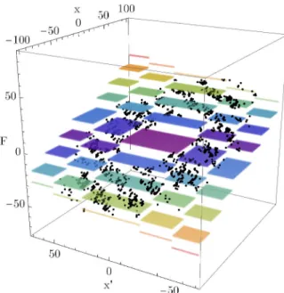
Fig. 8. Example trajectories of the micro-chaos map, leading to two separate attractors in case of ˆα=0.07, δ=0, ˆP =0.007, ˆD =0.02, ρI =0.001. Initial states:
x=0 and ∎: x′=4, ∎: x′= 8. Coloured layers show bands of same control effort valuesF.
Fig. 9. Example trajectory of the micro-chaos map, leading to a periodic cycle with chaotic oscillation superim- posed. ˆα= 0.07, δ =0, ˆP =0.007, ˆD =0.04, ρI =25.
Initial statex=0 and x′=10. Coloured layers show bands of same control effort valuesF.
5. CELL MAPPING RESULTS
Cell Mapping (Hsu, 1987) is a technique for the global analysis of dynamical systems. It involves discretization of a selected region of the state space (intocells), then one or more image cells – where the dynamics lead to – are determined for every cell.
In case of Simple Cell Mapping (scm), one image cell is determined for every cell, by starting a trajectory from the center of the cell, therefore the intermediate result ofscm
Fig. 10. Example trajectory of the micro-chaos map, leading to a chaotic attractor spanning over multiple control bands. ˆα = 0.07, δ = 0, ˆP = 0.4, ˆD = 0.25, ρI = 25. Initial state x = 0 and x′ = 150. Coloured layers show bands of same control effort valuesF. is a graph. By analysing that graph, one can determine periodic cycles (n-P groups consisting of n cells) and transient cells (which lead to a periodic group) forming the basin of attraction of periodic groups. The region outside the examined state space area is calledsink cell.
Utilizing scm, we have examined the state space of the micro-chaos map for variousρIvalues and realistic system parameters (ˆα=0.07, δ=0, ˆP =0.007, ˆD=0.02). As the ratio corresponding to the two resolutions increase, one can observe the transition from separate attractors to an enclosing periodic orbit with chaotic oscillations.
Figure 11. shows a case, when the output quantization is dominant, and there are six chaotic attractors in the state space. As the input quantization gains significance, the switching lines start to become jagged – resembling to a staircase or a zigzag – see Fig. 12. At this point the outermost chaotic attractors disappear due to a structural change in where the stable and unstable manifolds of the nearest saddle point intersect the jagged switching line.
Further increasing the value of ρI, the internal structure becomes a set of repellors and an enclosing periodic orbit appears, see Fig 13. The reason of this is the increased dead zone around thexaxis, which effectively means that the control is only proportional there.
6. CONCLUSION
We have presented themicro-chaos map corresponding to a digitally controlled inverted pendulum, with input and output quantization, and zero-order hold PD-control. The map itself shows colourful dynamical behaviour which is strongly related to the underlying patterns of control effort caused by the twofold quantization.
An important observation is, that the ratio of the quantizer resolutions has a critical value (ρ∗I, Eq. (7)), which corre- sponds to a special kind of bifurcation, where the corners ofjagged switching lines are touching each other, allowing the dynamics to bypass certain control effort values.
Cell Mapping methods were used to examine the state space during the variation of ρI and the transition from separate attractors to repellors surrounded by a chaotic attractor was shown. Cell mapping results enable us to qualitatively observe the resulting state space structure and determine the significance of the quantization(s) with respect to the applied control function.
ACKNOWLEDGEMENTS
The research leading to these results has received funding from the European Research Council under the European Union’s Seventh Framework Programme (FP7/2007-2013) ERC Advanced grant agreement№340889.
REFERENCES
Csern´ak, G., Gyebr´oszki, G., and St´ep´an, G. (2016). Multi- baker map as a model of digital PD control. Interna- tional Journal of Bifurcations and Chaos, 26(2), –.
Csern´ak, G. and St´ep´an, G. (2010). Digital control as source of chaotic behavior. International Journal of Bifurcations and Chaos, 5(20), 1365–1378.
Csern´ak, G. and St´ep´an, G. (2011). Sampling and round- off, as sources of chaos in PD-controlled systems. Pro- ceedings of the 19th Mediterranean Conference on Con- trol and Automation.
Csern´ak, G. and St´ep´an, G. (2012). Disconnected chaotic attractors in digitally controlled linear systems. Pro- ceedings of the 8th WSEAS International Conference on Dynamical Systems and Control, 97–102.
De Almeida, A.M.O. (1990). Hamiltonian systems: chaos and quantization. Cambridge University Press.
de Kraker, B., van der Spek, J.A.W., and van Campen, D.H. (2000). Extensions of cell mapping for discontinu- ous systems. In M. Wiercigroch and B. de Kraker (eds.), Applied Nonlinear Dynamics and Chaos of Mechanical Systems with Discontinuities, chapter 4, 61–102. World Scientific.
Gyebr´oszki, G. and Csern´ak, G. (2014). Methods for the quick analysis of micro-chaos. In J. Awrejcewicz (ed.), Applied Non-Linear Dynamical Systems, chapter 28, 383–395. Springer International Publishing.
Haller, G. and St´ep´an, G. (1996). Micro-chaos in digital control. Journal of Nonlinear Science, 6, 415–448.
Hsu, C. (1987). Cell-to-Cell Mapping: A Method of Global Analysis for Nonlinear Systems, volume 64 of Applied Mathematical Sciences. Springer, Singapore.
Nusse, H.E. and Yorke, J.A. (1996). Basins of attraction.
Science, 271, 1376–1380.
Widrow, B. and Koll´ar, I. (2008). Quantization Noise:
Roundoff Error in Digital Computation, Signal Process- ing, Control, and Communications. Cambridge Univer- sity Press, Cambridge, UK.
Zou, H. and Xu, J. (2009). Improved generalized cell map- ping for global analysis of dynamical systems.Science in China Series E: Technological Sciences, 52(3), 787–800.
Fig. 11. scmresult in case of ˆα=0.07,δ=0, ˆP =0.007, ˆD=0.02, ρI=0.1. There are 6 chaotic attractors highlighted with pink circles, their basin of attraction is coloured from left, to right along the xaxis:∎, ∎, ∎, ∎, ∎, ∎. The control bandsF are indicated with alternating shades. The fixed points are highlighted with white circles. Red ∎ colour indicates transient cells leading to the sink cell.
Fig. 12. scm result in case of ˆα= 0.07, δ= 0, ˆP = 0.007, ˆD = 0.02, ρI =2. There are 4 chaotic attractors (from left to right: ∎,∎, ∎, ∎), the leftmost and rightmost ones became repellors. The control bands F are indicated with alternating shades. It can be observed, that the switching lines become staircase like or fragmented. The control bandsF are indicated with alternating shades. Red∎colour indicates transient cells leading to the sink cell.
Fig. 13. scm result in case of ˆα= 0.07, δ = 0, ˆP =0.007, ˆD = 0.02, ρI = 64. It can be seen, that the method found some internal periodic groups without basin of attraction: these are the remains of the original attractor structure turning to repellors. The state space is attracted by a single periodic cycle coloured with ∎which encloses the internal structure. Red ∎colour indicates transient cells leading to the sink cell.