Stability and Sensitivity Analysis of Fuzzy Control Systems. Mechatronics Applications
Radu-Emil Precup, Stefan Preitl
“Politehnica” University of Timisoara, Dept. of Automation and Appl. Inform.
Bd. V. Parvan 2, RO-300223 Timisoara, Romania
Phone: +40-256-4032-29, -30, -24, -26, Fax: +40-256-403214 E-mail: radu.precup@aut.upt.ro, stefan.preitl@aut.upt.ro
Abstract: The development of fuzzy control systems is usually performed by heuristic means, incorporating human skills, the drawback being in the lack of general-purpose development methods. A major problem, which follows from this development, is the analysis of the structural properties of the control system, such as stability, controllability and robustness. Here comes the first goal of the paper, to present a stability analysis method dedicated to fuzzy control systems with mechatronics applications based on the use of Popov’s hyperstability theory. The second goal of this paper is to perform the sensitivity analysis of fuzzy control systems with respect to the parametric variations of the controlled plant for a class of servo-systems used in mechatronics applications based on the construction of sensitivity models. The stability and sensitivity analysis methods provide useful information to the development of fuzzy control systems. The case studies concerning fuzzy controlled servo-systems, accompanied by digital simulation results and real-time experimental results, validate the presented methods.
Keywords: Mamdani fuzzy controllers, stability analysis, sensitivity analysis, mechatronics, servo-systems.
1 Introduction
The development of fuzzy control systems (FCSs) is usually performed by heuristic means, due to the lack of general development methods applicable to large categories of systems. A major problem, which follows from the heuristic method of development, is the analysis of the structural properties of the control systems including the stability analysis and the sensitivity analysis with respect to the parametric variations of the controlled plant. In case of mechatronics applications focussed on servo-systems the analysis of these properties becomes more important due to the very good steady-state and dynamic performance they must ensure.
Therefore, the paper aims a twofold goal. Firstly, it presents one stability analysis method dedicated to FCSs applied to servo-systems with mechatronics applications,
involving the use of Popov’s hyperstability theory. Secondly, the paper performs the sensitivity analysis of FCSs with respect to the parametric variations of the controlled plant (CP) for a class of servo-systems based on the construction of sensitivity models. The considered FCSs contain Mamdani fuzzy controllers with singleton consequents, seen as type-II fuzzy systems [1, 2].
The stability analysis of an FCS is justified because only a stable FCS can ensure the functionality of the plant and, furthermore, the disturbance reduction, guarantee desired steady states, and reduce the risk of implementing the fuzzy controller (FC).
The main approaches in stability analysis of FCSs with Mamdani fuzzy controllers concern: the state-space approach based on a linearized model of the nonlinear system [3, 4], Popov’s hyperstability theory [5, 6], Lyapunov’s direct method [2, 7], the circle criterion [7, 8], the harmonic balance method [8, 9] referred to also as the describing function method [10, 11], the passivity approach [12], etc.
The sensitivity analysis of the FCSs with respect to the parametric variations of the CP is necessary because the behaviour of these systems is generally reported as
“robust” or “insensitive” without offering systematic analysis tools. The sensitivity analysis performed in the paper is based on the idea of approximate equivalence, in certain conditions, between FCSs and linear ones. This is fully justified because of two reasons. The first reason is related with the controller part of the FCS, where the approximately equivalence between linear and fuzzy controllers is generally acknowledged [13, 14]. The second reason is related with the plant part of the FCS.
The support for using an FC developed to control a plant having a linear or linearized model is in the fact that this plant model can be considered as a simplified model of a relatively complex model of the CP having nonlinearities or variable parameters or being placed at the lower level of large-scale systems. This is the case of servo-systems in mechatronics applications. Although the plant is nonlinear, it can be linearized in the vicinity of a set of operating points or of a trajectory. The plant model could be also uncertain or not well defined. The FC, as essentially nonlinear element, can compensate for the model uncertainties, nonlinearities and parametric variations of the CP. Fuzzy control must not be seen as a goal in itself, but sometimes the only way to initially approach the control of complex plants.
This paper is organized as follows. It will be treated in the following Section the stability analysis method based on the use of Popov’s hyperstability theory. The exemplification of the method is done by a case study regarding the FC development to control an electro-hydraulic servo-system. Then, in Section 3 an approach to the sensitivity analysis of the FCSs for a class of servo-systems with respect to the parametric variations of the CP is presented. This approach is illustrated by a case study regarding the fuzzy control of a nonlinear servo-system. Digital simulation results and real-time experimental results validate the presented approaches. The conclusions are drawn in the end of the paper.
2 Stability Analysis Method Based on Popov’s Hyperstability Theory
The SAM based on Popov’s hyperstability theory is applied to FCSs to control SISO plants when employing PI-fuzzy controllers (PI-FCs). The structure of the considered FCS is a conventional one, presented in Fig. 1 (a), where: r – the reference input, y – the controlled output, e – the control error, u – the control signal, d1, d2, d3 – the disturbance inputs.
Figure 1
Structure of FCS (a) and of PI-FC (b)
The CP includes the actuator and the measuring devices. The application of an FC, when conditions for linear operating regimes of the plant are validated, determines the FCS to be considered as a Lure-Postnikov type nonlinear control system (for example, see [15]). The PI-FC represents a discrete-time FC with dynamics, introduced by the numerical differentiation of the control error ek expressed as the increment of control error, Δek=ek–ek-1, and by the numerical integration of the increment of control signal, Δuk. The structure of the considered PI-FC is illustrated in Fig. 1 (b), where B-FC represents the basic fuzzy controller, without dynamics.
The block B-FC is a nonlinear two inputs-single output (TISO) system, which includes among its nonlinearities the scaling of inputs and output as part of its fuzzification module. The fuzzification is solved in terms of the regularly distributed (here) input and output membership functions illustrated in Fig. 2. Other distributions of the membership functions can modify in a desired way the controller nonlinearities.
Figure 2
Membership functions of input and output linguistic variables of B-FC
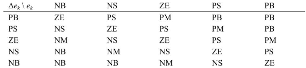
The inference engine in B-FC employs Mamdani’s MAX-MIN compositional rule of inference assisted by the rule base presented in Table 1, and the center of gravity method for singletons is used for defuzzification.
Table 1 Decision table of B-FC
Δek \ ek NB NS ZE PS PB
PB ZE PS PM PB PB PS NS ZE PS PM PB ZE NM NS ZE PS PM NS NB NM NS ZE PS NB NB NB NM NS ZE To develop the PI-FC the beginning is in the expression of the discrete-time equation of a digital PI controller in its incremental version:
)
( k k
P k I k P
k K e K e K e e
u = ⋅Δ + ⋅ = Δ + α⋅
Δ , (1)
where k is the index of the current sampling interval.
In case of a quasi-continuous digital PI controller the parameters KP, KI and α can be calculated as functions of the parameters kC (gain) and Ti (integral time constant) of a basic original continuous-time PI controller having the transfer function HC(s):
) 1 )](
/(
[ )
( C i i
C s k sT sT
H = + , (2)
and the connections between {KP, KI, α} and {kC, Ti} have the following form in the case of using Tustin’s discretization method:
) 2 /(
2 / , /
, )]
2 /(
1
[ s i I C s i I P s i s
C
P k T T K k T T K K T T T
K = − = α= = − , (3)
with Ts – the sampling period chosen in accordance with the requirements of quasi- continuous digital control.
The design relations for the PI-FC are obtained by the application of the modal equivalence principle [16] transformed into (4) in this case:
e I u e
e B B K B
BΔ =α , Δ = , (4)
where the free parameter Be represents designer’s option. Using the experience in controlling the plant one can choose the value of this parameter, but firstly it must be chosen to ensure the aim of a stable FCS.
The CP is supposed to be characterized by the following n-th order discrete-time SISO linear time-invariant state mathematical model (MM) including the zero-order hold:
k T k
k k
k
y
u x
c
b x A x
⋅
=
⋅ +
⋅
+1= , (5)
where: uk – the control signal; yk – the controlled output; xk – the state vector, dim xk
= (n,1); A, b, cT - matrices with the dimensions: dim A = (n, n), dim b = (n, 1), dim cT = (1, n).
To derive the stability analysis method it is necessary to transform the initial FCS structure into a multivariable one because the block B-FC in Fig.X.5 is a TISO system. This modified FCS structure is illustrated in Fig. 3 (a), where the dynamics of the fuzzy controller (its linearized part) is transferred to the plant (CP) resulting in the extended controlled plant (ECP, a linear one). The vectors in Fig. 3 (a) represent:
rk – the reference input vector, ek – the control error vector, yk – the controlled output vector, uk – the control signal vector. For the general use (in the continuous time, too) the index k may be omitted, and these vectors are defined as follows:
[ ] [ ]
k[
k k]
TT k k k T k k
k = r Δr e = e Δe y = y Δy
r , , , (6)
where Δvk = vk – vk-1 stands generally for the increment of the variable vk.
Figure 3
Modified structure of FCS (a) and structure used in stability analysis (b)
In relation with Fig. 3 (a), the block FC is characterized by the nonlinear input- output static map F:
T k
k f
R
R , ( ) [ ( ), 0]
: 2 2 F e e
F → = , (7)
where f ( f :R2 → R) is the input-output static map of the nonlinear TISO system B-FC in Fig. 1.
As it can be observed in (6), all variables in the FCS structure (in Fig. 3 (a)) have two components. This requires the introduction of a fictitious control signal, supplementary to the outputs of the block B-FC, for obtaining an equal number of inputs and outputs as required by the hyperstability theory in the multivariable case.
Generally speaking, the structure involved in the stability analysis of an unforced nonlinear control system (rk = 0 and the disturbance inputs are also zero) is presented in Fig. 3 (b). The block NL in Fig. 3 (b) represents a static nonlinearity due to the nonlinear part without dynamics of the block FC in Fig. 3 (a). The connections between the variables of the control system structures in Fig. 3 are:
k k k k
k u F e y e
v =− = − ( ), = − , (8)
with the second component of F being always zero to neglect the effect of the fictitious control signal.
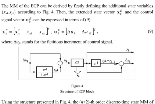
The MM of the ECP can be derived by firstly defining the additional state variables {xuk,xyk} according to Fig. 4. Then, the extended state vector xkE and the control signal vector ukE can be expressed in terms of (9):
[ ] [
k fk]
TE k T yk uk T k E
k = x x x u = Δu Δu
x , , (9)
where Δufk stands for the fictitious increment of control signal.
Figure 4 Structure of ECP block
Using the structure presented in Fig. 4, the (n+2)-th order discrete-time state MM of the ECP becomes (10):
E k E E k
E k E E k E E k
x C y
u B x A x
⋅
=
⋅ +
⋅
+1= , (10)
with the matrices AE (dim AE = (n+2,n+2)), BE (dim BE = (n+2,2)) and CE (dim CE
= (2,n+2)) expressed as follows:
⎥⎦
⎢ ⎤
⎣
⎡
= −
⎥⎥
⎥
⎦
⎤
⎢⎢
⎢
⎣
⎡
=
⎥⎥
⎥
⎦
⎤
⎢⎢
⎢
⎣
⎡
= 0 1
0 0
, 1 0
1 1
, 0 0
0
1 E E TT
T T E
c C c 1 b B c
0
0 b A
A . (11)
Then, the second equations in (8) and (10) can be transformed into the following equivalent expressions:
k b k k E
k C x x C e
e = − ⋅ , = ⋅ , (12)
where the matrix Cb, dim Cb = (n+2,2), can be calculated relatively easy as function of CE.
The main part of the proposed stability analysis method can be stated in terms of the following theorem giving sufficient stability conditions.
Theorem 1. The nonlinear system, with the structure presented in Fig. 3 (b) and the MM of its linear part (10), is globally asymptotically stable if:
- the three matrices P (positive definite, dim P = (n+2,n+2)), L (regular, dim L = (n+2,n+2)) and V (any, dim V = (n+2,2)) fulfill the requirements (13):
V V B P B
L V A P B C
L L A P A
⋅
=
⋅
⋅
−
⋅
=
⋅
⋅
−
⋅
−
=
⋅
⋅
T E T
E
T T E T
E E
T E
T E
) (
) ( ) (
, (13)
- introducing the matrices M (dim M = (2,2)), N (dim N = (2,2)) and R (dim R = (2,2)) defined in terms of (14):
V V R
C B
P A
V L C
N
C P L L C
M
⋅
=
−
⋅
⋅
−
⋅
⋅
=
⋅
−
⋅
⋅
=
T
T E E
T E T
b
b T
T b
] ) ( 2 )
( [
) (
) (
) (
, (14)
the Popov-type inequality (15) holds for any value of the control error ek: 0
) ( )
( k ⋅ T ⋅ k + k T ⋅ ⋅ k ≥
f e n e e M e , (15)
where n represents the first column in N.
The proof of Theorem 1, based on the Kalman-Szegö lemma [17] and on processing the Popov sum, is presented in [18] for the PI-FCs with prediction.
By taking into account these aspects, the stability analysis method dedicated to FCSs with PI-FCs consists of the following steps:
- step (a): express the MM of the CP, choose the sampling period Ts and calculate the discrete-time state-space MM of the CP with the zero-order hold, (5),
- step (b): derive the discrete-time state-space mathematical model of the ECP, (10),
- step (c): compute the matrix Cb in terms of (12),
- step (d): solve the system of equations (13), with the solutions P, L and V, and calculate the matrices M, N and R in (14),
- step (e): set the value of the free parameter Be > 0 of the PI-FC, and tune the other parameters of the PI-FC in terms of (4),
- step (f): check the stability condition (15) for any values of PI-FC inputs in operating regimes considered to be significant for FCS behaviour.
To test the presented stability analysis method it is considered the CP of an electro- hydraulic servo-system (EHS) used as actuator in mechatronics applications, with the structure presented in Fig. 5 (a) [19], where: NL 1 … NL 5 – nonlinearities, EHC – electro-hydraulic converter, SVD – slide-valve distributor, MSM – main
servo-motor, M 1 and M 2 – measuring devices; u – control signal, y – controlled output; x1 and x2 – state variables; x1M and x2M – measured state variables, ul = 10 V, g0 = 0.0625 mm/V, ε2 = 0.02 mm, ε4 = 0.2 mm, x1l = 21.8 mm, yl = 210 mm, Ti1 = 0.001872 sec, Ti2 = 0.0756 sec, kM1 = 0.2 V/mm, kM2 = 0.032 V/mm. To obtain a relatively simple FC, the CP is represented here by the stabilized electro-hydraulic servo-system (SEHS), and the FCS structure is presented in Fig. 5 (b).
Figure 5
Structure of EHS as CP (a) and structure of FCS (b)
The SEHS represents itself a state feedback control system, with AA – adder amplifier, and kx1, kx2, kAA – parameters of the state feedback controller. By omitting the nonlinearities of the EHS, imposing the double pole of the SEHS in −1, the pole placement method leads to the transfer function of the SEHS block, HCP(s):
2 2
2 0 2 1 2 2 1 2 1
2
) 1 (
1 )]
/(
[ )]
/(
[ 1
/ ) 1
( k T k k k k s TT gk k s s
s k H
M AA i i x M AA x i M
x
CP = +
+
= + , (16)
obtained for kx1 = 0.2997, kx2 = 1, kAA = 0.0708.
The steps of the stability analysis method have been proceeded, but only the values of M and nT are presented because these two matrices appear in the stability condition (15), tested by digital simulation:
[
0.9855 0]
0 , 0
0 0071 .
2 ⎥ =
⎦
⎢ ⎤
⎣
=⎡ nT
M , (17)
and the parameters of the PI-FC ensuring the stability of the FCS have been tuned as: Be = 0.3, BΔe = 0.0076, BΔu = 0.0203. To verify the stability of all FCS the dynamic behaviour of the free control system was simulated, when the system
started from two different, arbitrarily chosen, initial states, obtained by feeding a d3=–0.5 and a d3=–1.5 disturbance input according to Fig. 1 (a). The FCS behaviour is presented in Fig. 6, and it illustrates that the FCS analyzed by using the presented SAM is stable.
Figure 6
FCS behaviour for d3 = − 0.5 (a) and d3 = − 1.5 (b)
3 Sensitivity Analysis of a Class of Fuzzy Control Systems. Case Study
Let the considered control system structure be a conventional one, presented in Fig.
7 (a), where: C – controller, CP – controlled plant, RF – the reference filter, r – reference input, r~ – filtered reference input, e – control error, u – control signal, y – controlled output, d1, d2, d3, d4 – disturbance inputs. Depending on the place of feeding the disturbance inputs to the CP and on the CP structure, the accepted types of disturbance inputs {d1, d2, d3, d4} are defined in terms of Fig. 7 (b).
Figure 7
Control system structure (a) and disturbance inputs types (b)
The class of plants with the simplified structure illustrated in Fig. 7 (a), is considered to be linearized around a steady-state operating point and characterized by the transfer function HP(s):
)]
1 ( /[
)
(s k s T s
HP = P + Σ , (18)
with kP – gain and TΣ – small time constant or sum of all parasitic time constants, belongs to a class of integral-type systems with variable parameters in case of servo- systems with mechatronics applications.
For these plants, it is recommended the use of linear PI controllers having the transfer function HC(s) in (2) with kC =kcTi. Based on the Extended Symmetrical Optimum (ESO) method [19], the parameters of the controller {kc (or kC) – controller gain, Ti – integral time constant} are tuned in terms of (19) guaranteeing the desired control system performance by means of a single design parameter, β:
) /(
1 ,
), /(
1 β3/2 Σ2 =β Σ = β1/2 Σ
= k T T T k k T
kc P i C P . (19)
The PI controllers can be tuned also in terms of the Iterative Feedback Tuning (IFT) method, representing a data-based design method where the update of the controller parameters is done through an iterative procedure. IFT is a gradient-based approach, based on input-output data recorded from the closed-loop system. The control system performance indices are specified by the proper expression of a criterion function. Optimizing such functions usually requires iterative gradient-based minimization, and this can be a complicated function of the plant and of the disturbances dynamics. The key property of IFT is that the closed-loop experimental data are used to calculate the estimated gradient of the criterion function. Several experiments are performed at each iteration and, based upon the input-output data collected from the system, the updated controller parameters are obtained.
Theoretical and practical applications of IFT have been reported in [20, 21, 22, 23].
Using the IFT as a design step in the development of fuzzy controllers can result in efficient development techniques for fuzzy controller with dynamics.
According to [24], the variation of CP parameters ({kP, TΣ} for the considered class of CPs) due to the change of the steady-state operating points or to other conditions leads to additional motion (of the control systems). This motion is usually undesirable under uncontrollable parametric variations. Therefore, to alleviate the effects of parametric disturbances it is necessary to perform the sensitivity analysis with respect to the parametric variations of the CP.
It is generally accepted that FCs ensure control system performance enhancement with respect to the modifications of the reference input, of the load disturbance inputs or to parametric variations. This justifies the research efforts focused on the systematic analysis of FCSs behaviour with respect to parametric variations and the need to perform the sensitivity analysis with this respect that enables to derive sensitivity models for the FCs and for the overall FCSs.
The sensitivity models enable the sensitivity analysis of the FCSs accepted, as mentioned in Section 1, to be approximately equivalent with the linear control systems. This justifies the approach to be presented in the sequel, that the sensitivity models of the FCSs are approximately equivalent to the sensitivity models of the linear ones. Therefore, it is necessary to obtain firstly the sensitivity models of the linear control system in Fig. 7 (a).
Defining the state sensitivity functions {λ1, λ2, λ3} and the output sensitivity function, σ, there have been derived several sensitivity models, four of them being presented as follows:
- with respect to the variation of kP, the step modification of r, and d3(t) = 0:
), ( ) (
), ( )]
/(
1 [ ) (
), ( )]
/(
1 [
) ( )]
/(
1 [ ) ( )]
/(
1 [
) ( )]
/(
1 [ ) ( ) / 1 ( ) ( )]
/(
1 [ ) (
), ( ) (
1
1 0 3
0 2
0 0 2 / 1
30 2
0 0 2 / 1 10
2 0 0 2 / 1
3 2
0 2 / 1 2
0 1
2 0 2 / 1 2
2 1
t t
t T t
t r T k
t x T k t
x T k
t T
t T t
T t
t t
P
P P
λ σ
λ β λ
β
β β
λ β
λ λ
β λ
λ λ
=
−
= +
+ +
−
− +
−
−
=
=
Σ Σ
Σ Σ
Σ Σ
Σ
(20)
- with respect to the variation of TΣ, the step modification of r, and d3(t) = 0:
), ( ) (
), ( )]
/(
1 [ ) (
), ( )]
/(
1 [
) ( )]
/(
1 [ ) ( ) / 1 ( ) ( )]
/(
1 [
) ( )]
/(
1 [ ) ( ) / 1 ( ) ( )]
/(
1 [ ) (
), ( ) (
1
1 0 3
0 3
0 2 / 1
30 3
0 2 / 1 20
2 0 10
3 0 2 / 1
3 2
0 2 / 1 2
0 1
2 0 2 / 1 2
2 1
t t
t T t
t r T
t x T t
x T t
x T
t T t
T t
T t
t t
λ σ
λ β λ
β
β β
λ β
λ λ
β λ
λ λ
=
−
=
−
−
− +
+
+ +
−
−
=
=
Σ Σ
Σ Σ
Σ
Σ Σ
Σ
(21)
- with respect to the variation of kP, the step modification of d3, and r(t) = 0:
), ( ) (
), ( )]
/(
1 [ ) (
), ( )]
/(
1 [ ) ( )]
/(
1 [ ) (
), ( ) / 1 (
) ( ) / 1 ( ) ( ) / ( ) ( ) / 1 ( ) (
1
1 0 3
3 0 0 2 / 1 1
0 0 2 / 1 2
30 0
20 0 2
0 0 1
0 1
t t
t T t
t T k t
T k t
t d T
t x T t T k t T t
P P
P
λ σ
λ β λ
λ β
λ β
λ
λ λ
λ
=
−
=
+
−
= +
+ +
+
−
=
Σ
Σ Σ
Σ
Σ Σ
Σ
(22)
- with respect to the variation of TΣ, the step modification of d3, and r(t) = 0:
).
( ) (
), ( )]
/(
1 [ ) (
), ( )]
/(
1 [ ) ( )]
/(
1 [ ) (
), ( ) / ( ) ( ) / (
) ( ) / 1 ( ) ( ) / ( ) ( ) / 1 ( ) (
1
1 0 3
3 0 0 2 / 1 1
0 0 2 / 1 2
30 2
0 0 20
2 0 0
10 2
0 2
0 0 1
0 1
t t
t T t
t T k t
T k t
t d T k t x T k
t x T t T k t T t
P P
P P
P
λ σ
λ β λ
λ β
λ β
λ
λ λ
λ
=
−
=
+
−
=
−
−
− +
+
−
=
Σ
Σ Σ
Σ Σ
Σ Σ
Σ
(23)
The behaviours of these four sensitivity models, for the unit step modification of r followed by a unit step modification of d3 after 250 sec, starting with the initial conditions λ1(0) = 2, λ2(0) = 1, λ3(0) = 0, are shown in Fig. 8.
Figure 8
Behaviour of sensitivity models (20) (in (a)), (21) (in (b)), (22) (in (c)) and (23) (in (d))
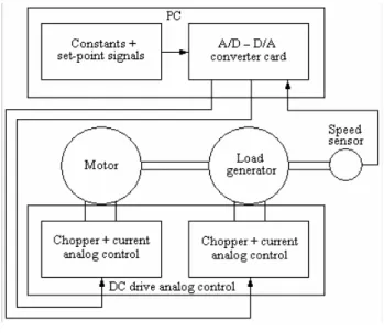
The PI-FC development method which can be expressed by using the stability and sensitivity analyses presented in this paper is applied in case of a nonlinear laboratory DC drive, AMIRA DR300.
The DC motor is loaded using a current controlled DC generator, mounted on the same shaft, and the drive has built-in analog current controllers for both DC machines with rated speed of 3000 rpm, rated power equal to 30 W, and rated
current equal to 2 A. The speed control of the DC motor is digitally implemented using an A/D – D/A data converter card. The speed sensors are a tacho generator and an additional incremental rotary encoder mounted at the free drive-shaft.
The schema of the experimental setup is presented in Fig. 9.
In these conditions, the speed response of the FCS with RF and PI-FC with respect to the modification of the reference input and without load is presented in Fig. 10.
Due to the integral feature of the PI-fuzzy controller structure it is not necessary to present the control system behaviour with respect to the modifications of the load disturbance inputs.
Figure 9 Experimental setup schema
Figure 10
Speed response of FCS without load
Conclusions
The paper presents one stability analysis method and performs the sensitivity analysis of fuzzy control systems with Mamdani fuzzy controllers dedicated to control of servo-systems in mechatronics applications.
The presentation is focused on PI-fuzzy controllers, but it can be applied with no major problems in case of PD- or PID-fuzzy controllers and of complex fuzzy controller structures as well [25, 26, 27].
The methods can be formulated under the form of useful design recommendations for the fuzzy controllers.
The case studies presented in the paper, accompanied by digital simulation results and by experimental results, validate the theoretical approaches.
References
[1] Kóczy, L. T.: Fuzzy If … Then rule models and their transformation into one another, IEEE Transactions on Systems, Man, and Cybernetics - Part A, 1996, Vol. 26, pp. 621-637
[2] Sugeno, M.: On stability of fuzzy systems expressed by fuzzy rules with singleton consequents, IEEE Transactions on Fuzzy Systems, 1999, Vol. 7, pp. 201-224
[3] Aracil, J., A. Ollero, and A. Garcia-Cerezo: Stability indices for the global analysis of expert control systems, IEEE Transactions on Systems, Man, and Cybernetics, 1989, Vol. 19, pp. 998-1007
[4] Precup, R.-E., S. Doboli, and S. Preitl: Stability analysis and development of a class of fuzzy control systems, Engineering Applications of Artificial Intelligence, 2000, Vol. 13, pp. 237-247
[5] Opitz, H.-P.: Fuzzy control and stability criteria, Proceedings of First EUFIT’93 European Congress, Aachen, Germany, 1993, Vol. 1, pp. 130- 136
[6] Precup, R.-E. and S. Preitl: Popov-type stability analysis method for fuzzy control systems, Proceedings of Fifth EUFIT’97 European Congress, Aachen, Germany, 1997, Vol. 2, pp. 1306-1310
[7] Passino, K. M. and S. Yurkovich: Fuzzy Control, Addison Wesley Longman, Inc., Menlo Park, CA, 1998
[8] Driankov, D., H. Hellendoorn and M. Reinfrank: An Introduction to Fuzzy Control, Springer-Verlag, Berlin, Heidelberg, New York, 1993
[9] Kiendl, H.: Harmonic balance for fuzzy control systems, Proceedings of First EUFIT’93 European Congress, Aachen, Germany, 1993, Vol. 1, pp.
137-141
[10] Ying, H.: Analytical structure of a two-input two-output fuzzy controller and its relation to PI and multilevel relay controllers, Fuzzy Sets and Systems, 1994, Vol. 63, pp. 21-33
[11] Gordillo, F., J. Aracil and T. Alamo: Determining limit cycles in fuzzy control systems, Proceedings of FUZZ-IEEE’97 Conference, Barcelona, Spain, 1997, pp. 193-198
[12] Calcev, G.: Some remarks on the stability of Mamdani fuzzy control systems, IEEE Transactions on Fuzzy Systems, 1998, Vol. 6, pp. 436-442 [13] Tang, K. L. and R. J. Mulholland: Comparing fuzzy logic with classical
controller designs, IEEE Transactions on Systems, Man, and Cybernetics, 1987, Vol. 17, pp. 1085-1087
[14] Moon, B. S.: Equivalence between fuzzy logic controllers and PI controllers for Single Input systems, Fuzzy Sets and Systems, 1995, Vol.
69, pp. 105-113
[15] Hill, D. J. and C. N. Chong: Lyapunov functions of Lure-Postnikov form for structure preserving models of power plants, Automatica, 1989, Vol.
25, pp. 453-460
[16] Galichet, S. and L. Foulloy: Fuzzy controllers: synthesis and equivalences, IEEE Transactions on Fuzzy Systems, 1995, Vol. 3, pp. 140-148
[17] Landau, I. D.: Adaptive Control, Marcel Dekker, Inc., New York, 1979 [18] Precup, R.-E., S. Preitl, and G. Faur: PI predictive fuzzy controllers for
electrical drive speed control: methods and software for stable development, Computers in Industry, 2003, Vol. 52, pp. 253-270
[19] Preitl, S. and R.-E. Precup: An extension of tuning relations after Symmetrical Optimum method for PI and PID controllers, Automatica, 1999, Vol. 35, pp. 1731-1736
[20] Hjalmarsson, H., S. Gunnarsson, and M. Gevers: A convergent iterative restricted complexity control design scheme, Proceedings of the 33rd IEEE Conference on Decision and Control, Lake Buena Vista, FL, 1994, pp.
1735-1440
[21] Hjalmarsson, H., M. Gevers, S. Gunnarsson, and O. Lequin: Iterative Feedback Tuning: theory and applications, IEEE Control Systems Magazine, 1998, Vol. 18, pp. 26-41
[22] Lequin, O., M. Gevers, M. Mossberg, E. Bosmans, and L. Triest: Iterative Feedback Tuning of PID parameters: comparison with classical tuning rules, Control Engineering Practice, 2003, Vol. 11, pp. 1023-1033
[23] Hamamoto, K., T. Fukuda, and T. Sugie: Iterative Feedback Tuning of controllers for a two-mass-spring system with friction, Control Engineering Practice, 2003, Vol. 11, pp. 1061-1068
[24] Rosenwasser, E. and R. Yusupov: Sensitivity of Automatic Control Systems, CRC Press, Boca Raton, FL, 2000
[25] Kovács, Sz. and L. T. Kóczy: Application of an approximate fuzzy logic controller inan AGV steering system, path tracking and collision avoidance strategy, Fuzzy Set Theory, Tatra Mountains Mathematical Publications, 1999, Vol. 16, pp. 456-467
[26] Tar, J. K., I. J. Rudas, J. F. Bitó, L. Horváth, and K. Kozlowski: Analysis of the effect ot backlash and joint acceleration measurement noise in the adaptive control of electro-mechanical systems, Proceedings of the ISIE 2003 International Symposium on Industrial Electronics, Rio de Janeiro, Brasil, 2003, CD issue, file BF-000965.pdf
[27] Vaščák. J. and L. Madarász: Automatic adaptation of fuzzy controllers, Acta Polytechnica Hungarica, 2005, Vol. 2, No. 2, pp. 5-18