Development of Conventional and Fuzzy Controllers and Takagi-Sugeno Fuzzy Models Dedicated for Control of Low Order Benchmarks with Time Variable Parameters

Development of Conventional and Fuzzy

Controllers and Takagi-Sugeno Fuzzy Models Dedicated for Control of Low Order

Benchmarks with Time Variable Parameters

Stefan Preitl

, Radu-Emil Precup

, Zsuzsa Preitl

* “Politehnica” University of Timisoara, Dept. of Automation and Appl. Inform.

Bd. V. Parvan 2, RO-300223 Timisoara, Romania

Phone: +40-256-4032-29, -30, -24, -26, Fax: +40-256-403214 E-mail: spreitl@aut.utt.ro, rprecup@aut.utt.ro

** Budapest University of Technology and Economics, Dept. of Automation and Applied Informatics, MTA-BME Control Research Group

Goldmann Gy. tér 3, H-1111, Budapest, Hungary; fax : +36-1-463-2871 E-mail : preitl@aut.bme.hu

Abstract: The paper presents development and tuning tehniques and solutions for PI and PID controllers, and Takagi-Sugeno fuzzy controllers with PI and PID type dynamics meant for applications which can be characterised with low order benchmark type modeles (for example electrical and hydraulic driving and positioning systems).Two type of plants and two control structures with homogenous and with non-homogenous information processing with respect to the inputs are presented, including tuning and optimization aspects. Then Takagi-Sugeno fuzzy models dedicated to a class of plants characterized by Two Input- Single Output linear time-varying systems are presented. It is offered a stability test algorithm of the fuzzy control systems involving Takagi-Sugeno fuzzy controllers, to control the accepted class of plants. The tuning methods are briefly presented in relation with a control solution for a drive system with a variable inertia strip winding system.

Keywords: Controllers with PI and PID dynamics, Takagi-Sugeno fuzzy models, Takagi- Sugeno fuzzy controllers, stability analysis, winding system.

1 Introduction

Take the class of plants (P) having the transfer functions expressed as:

) 1

) (

( = +

sT s

s k

H_P ^P (a),

) 1 )(

1 ) (

( = + +

sT sT

s k

H_P ^P (b) (1.1)

) 1 )(

1 ) ( (

1 + Σ

= +

sT sT

s s k

H_P ^P (a),

) 1 )(

1 )(

1 ) ( (

2

1 + + Σ

= +

sT sT sT s k

H_P ^P (b). (1.2)

The parametres kP can be constant or variable, and it is asumed that TΣ < T2 <(<<) T1; this class of models characterize well enough electrical and hydraulic driving and possitioning systems (control of possition and drive applications as controlled plants) [1], [2], [6].

The paper’s aim is to develop Takagi-Sugeno (TS) fuzzy controllers (FCs) based on classical development methods, meant for position control of electrical and hydraulic drives with linear constant or time-varying (LTV) parameters characterized by benchmark type models of form (1) and (2). If the parameters are continuously varying, the LTV systems may result as linearized nonlinear systems in the vicinity of a set of operating points or of an operating trajectory.

These features determine the wide application area of robust control, adaptive control and TS fuzzy models. Regarded to the use of TS fuzzy models, the application is based in spite of their drawbacks such as:

- The behavior of the global TS fuzzy model can significantly divert from the expected behavior obtained by the merge of the local models;

- The stability analysis and testing of fuzzy control systems based on TS fuzzy models is relatively difficult, because of the complex aggregation of the local models in the inference engine.

Firstly, the paper presents two classical development procedures for continuously and quasi-continuously working PI and PID controllers, based on extensions of the widely used Symmetrical Optimum Method (Section 2). Then, a class of TS models for Two Input-Single Output (TISO) LTV plants is presented (Section 3).

In Section 4 there are defined the TS fuzzy controllers meant for controlling the TS fuzzy models. Based on these, a stability test algorithm is presented (based on Lyapunov’s stability theory) for a class of fuzzy systems with TS fuzzy controllers controlling the TISO LTV plants (Section 5). Results concerning the development of conventional and fuzzy control solutions for a drive system with two output coupled motors, applicable to the rolls of a hot rolling mill and to a variable inertia strip winding system, are presented in Section 6. Section 7 is focused on the concluding part of the paper.

2 Development of Continuously and Quasi- Continuously Operating PI and PID Control Algorithms

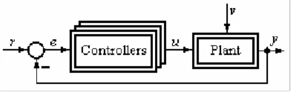
Many control applications prefer structures with typical control algorithms with homogenous or non-homogenous information processing on the two input channels [1], [3], [4]. Such structures have the general form given in Fig. 2.1-a -b and -c presents some particular control laws regarding the inputs. The blocks (1) ...

(5) can be described by its specific transfer functions (t.f.s); w(t) or r(t) – the reference signal (or the filtered refernce signal), y(t) - the measured output, u(t) - the control signal (or its components, with index), e(t) - the control error.

There can be established relations between such controllers and the 2-DOF controllers [3]. For example, a block diagram of a 2-DOF control structure is presented in figure 2.2. R(z) , S(z) and T(z) are the characteristic blocks of the 2- DOF controller, P is the plant; v1(t), v2(t) – plant disturbances.

Figure 2.1

Typical I-DOF controller structures and particularization

Figure 2.2

Structure of the 2-DOF controller.

The 2-DOF controller can be restructured in different ways; for the given low order plants – from a practical point of view – the presence of a conventional

controller (particularly PI or a PID and signal filters) can be highlighted. Two types of structures are detailed in figure 2.3. These rearrangements allow:

- to take over design experience from case of PI and PID controllers;

- an easy introduction of supplementary blocks specific to PI and PID controllers (Anti Windup circuit, bumpless switching and others);

- the transformation of PI and PID controllers into 2 DOF structures and vice versa.

The controllers in figure 2.3 will be characterized – for example – by continuous t.f.s C(s), CF(s), C^*(s), CP(s), in which the parallel realisation tuning parameters are highlighted{kC, Ti, Td, Tf}; discretizing, the digital control algorithm is obtained. Taking the basic controller C(s) of PID type, it can be written:

- for the basic PID structure in Fig. 2.1 (b) (parallel form):

; ) 1 1 (

) 1 (

) 1 ) ( 1 ( 1 ) (

) ) ( ( , 1 ) 1 1

) ( (

) ) (

( ₂

2

*

f d i i

f d i i

f d i C

sT s T s T T

sT s T s T

T s

r s s r sT F sT k sT

s e

s s u C

+ + +

+ + −

− +

= + =

+ +

=

=

α β

(2.1)

Figure 2.3

Two alternatives for rearranging a 2 DOF controller.

- for the structure (a) in figure 2.3:

; 1 )

) ( (

) ) (

( , 1 ) 1 1

) ( (

) ) ( (

f d R

f F

f d i

R sT

k sT s r

s s u sT C

sT k sT

s e

s s u

C = = + +

+ + +

=

= α β ^(2.2)

- for the structure (b) in figure 2.3 (with the notation C(s)=C^*(s)):

. 1 ) ) (

( ) ) ( ( , 1 ] ) 1 1 ( ) 1 ) [(

( ) ) ( (

f d R

f P f d i

R sT

k sT s r

s s u sT C sT k sT

s e

s s u

C = = + +

− + + +

−

=

=

∗ α β α β ^(2.3)

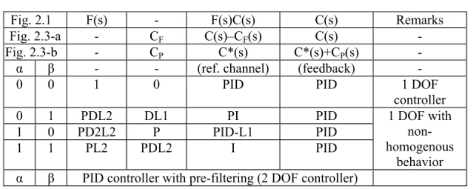
Table 2.1

Connections between 2 DOF controller and extended 1 DOF controller structure.

Fig. 2.1 F(s) - F(s)C(s) C(s) Remarks

Fig. 2.3-a - C_F C(s)–C_F(s) C(s) -

Fig. 2.3-b - CP C*(s) C*(s)+CP(s) -

α β - - (ref. channel) (feedback) -

0 0 1 0 PID PID 1 DOF

controller

0 1 PDL2 DL1 PI PID

1 0 PD2L2 P PID-L1 PID

1 1 PL2 PDL2 I PID

1 DOF with non- homogenous

behavior α β PID controller with pre-filtering (2 DOF controller)

Remarks: P – proportional, D – derivative, L – lag, I – integrator modules.

Depending on the values of α and β parameters, for the presented blocks the behaviors from in Table 2.1 are obtained.

The choice of a certain representation of the controller depends on [3]:

- the structure of the available controller;

- the adopted algorithmic design method, and the result of this design.

In the presence of an integral (I) component and a limitation block in the controller structure, figure 2.4 (a), the use of the AWR measure (Anti-Windup- Reset) is recommended. A classical structure for introducing the AWR measure on a controller structure with integral component is presented in figure 2.4 (b). The AWR measure can be globally implemented with respect to controller output or locally, with respect to integral (I) component of the controller.

Figure 2.4

Classical structure for introducing ARW measure on the controller structure The transfer functions of the continuous PI (PID) controllers are written related to the design procedure and the implementation (discretization) procedure. For the serial form of PI and PID controllers the t.f.s are:

PI: {kc, Tc}

( )

( 1 sT

) s

s k

C = +

PID: {kc, Tc, Tc’}

( )

( 1 sT

)( 1 sT

) s

s k

C = + +

The implementation of a quasi-continuously (QC) operating PID digital control algorithm can be based on the informational diagram presented in figure 2.5; the appearance of a supplementary state variables xk, is associated to integral (I) component and the adding of the AWR measure. The parameter values {Kpid, Ki , Kd ,Karw} depends on the continuous parameters {kr, Tr, Tr’} and on the sampling time value, Te .

Figure 2.5

Quasi-continuously operating PID digital control algorithm implementation.

The implementation of non-homogenous information processing (Fig. 2.1-c) has two requirements [3], [4]:

- an I or PI behavior with respect to the reference channel;

- a PI or PID behavior with respect to the feedback channel. The non- homogenous information processing structure respects the following informations (Table 2.2).

Table 2.2

Transfer functions of blocks in Fig. 2.1-c (parallel form)

Case Channel Block 3 Block 4 Block 5 Type w, (r) I: (1/sTi) ---- P: (kC) I: (1/sTi) (1)

y I: (1/sT_i) P: (1) P: (k_C) PI: (1+1/sT_i) w, (r) PI: (1+1/sTi) ---- P: (kC) PI: (1+1/sTi) (2)

y PI: (1+1/sTi) D: (sTd) P: (kC) PID

In order to avoid difficulties due to contradictory results obtained from design according to reference tracking and disturbance rejection, different optimal - or in special cases, optimal-like tuning techniques can be adopted. Two of these methods are considered here to be representative:

- the Modulus Optimum method, (MO-m), [1],

- the Symmetrical Optimum method (SO-m) [1] and two modified (extended versions, the Extended Symmetrical Optimum method (ESO-m) [2] and the

“extended” (modified version) of the extended Symmetrical Optimum method (2E-SO-m)Criterion. The main advantage of this ESO-m and 2E-SO- m consist in the possibility to increase the control system phase reserve and – for specific cases – in a better load disturbance rejection.

The controller parameters – in its serial form – can be calculated using the relations synthetised in Table 2.3. The design parameter β belongs usually to the domain 4 ≤ β ≤ 16.

In the case of implementation, the problem of bump-less transfer from one local crisp controller to another is solved in a crisp manner, exemplified here for two local controllers of digital PI-type, the “old” one with the parameters {q1, q0}, and the “new” one with the parameters {q1*, q0*}:

*1 0* 1* 1 1

0 1

1 ₋ , _{− −}

− + + = + +

= _{k k k k k k k}

k u q e q e u u q e q e

u . (2.6)

It is necessary to compute previously “past values” which are necessary to the new controller. As it can be observed in (16), ek-1* represent these new initial conditions (the past values).

3 A Class of Takagi-Sugeno Fuzzy Models

The following Takagi-Sugeno fuzzy model to represent a TISO LTV system will be used that models the controlled plant [7]:

Table 2.3

Tuning relations after [2], [6]

P(s) Contr.

type Tuning relations

0 1 2

) 1 ( +sT_Σ s

k_{p PI}

{kc, Tc}

Σ Σ

=

= T T

T k k

c

p c

β β^{3/2 2}

1

(ESO-m.[2])

) 1 )(

1

( +sT₁ +sT_Σ s

k_{p PID}

{kc, Tc, Tc’}

1 ,

2 2 / 3

, 1

T T T T

T k k

c c

p r

=

=

=

Σ Σ

β

β (ESO-m[2])

1

2 1 T T

T k k

c

p c

=

=

Σ (MO-m)

) 1 )(

1

( +sT₁ +sT_Σ k_P , m = TΣ/T1

PI {kc, Tc}

(1+m)²

kc = ––––––––––––– , β^3/2 ·kP ·TΣ'·m

β TΣ' ∆m(m) (2E-SO-m) Tc= ––––––––––– [6]

(1 + m)²

∆m(m)=1+(2-β^1/2)m+m²

2 ' 1 , 2

1

T T T T

T k k

c c

p c

=

=

=

Σ (MO-m)

) 1 )(

1 )(

1

( +sT₁ +sT₂ +sT_Σ k_P

m = TΣ/T1

PID {kc, Tc, Tc’}

(1+m)²

kc = ––––––––––––– , Tc’=T2

β^3/2 ·kP ·TΣ'·m

β TΣ' ∆m(m) (2E-SO-m) Tc= ––––––––––– [6]

(1 + m)²

∆m(m)=1+(2-β^1/2)m+m²

, 1 ), ( ) ( ) ( ) ( ) ( THEN

is ) ( AND AND is ) ( AND is ) ( IF

: _{1 1 2 2}

m l

s v s P s u s P s y

F t z F

t z F

t z R

v l u

l

l n n

l l

l

K K

= +

= ^(3.1)

where:

u(s), v(s), y(s) – the Laplace transform of the plant input (the control signal) u(t), of the disturbance input v(t) and of the controlled output y(t);

R^l – the lth inference rule, l = 1 … m; m – the number of inference rules;

zi(t) – the measurable plant variables, i = 1 … n, and:

T n t z t z t z

t) [ ( ) ( ) ( )]

( = _{1 2} K

z ; (3.2)

n – the number of measurable plant (system) variables pointing out the time- variation of the plant;

F^l – the linguistic terms associated to the measurable variable zⁱ(t) and to the rule R^l;

P

(s )

P

(s )

The TS fuzzy model (3.1) includes both the inference rules as part of the rule base and the local analytic models of the TISO LTV system. The controlled output is inferred by taking the weighted average of all local models appearing in (3.1), which characterizes the properties of the controlled plant in a local region of the input space; so it is referred to as fuzzy dynamic local model [8], [9]. The following notation is introduced:

m l

t

t _l

l( )=µ ( ()), =1K

µ z , (3.3)

for the membership degrees of the normalized membership functions µl of the inferred fuzzy set F^l, where:

m l

F

F ⁿ

i l i

l I , 1K

1 =

= = , (a) and ( ) 1

1 =

∑ µ= m

l l t . (b) (3.4)

By using the product inference method in (3.4) (b) and the weighted average method for defuzzification, the TS fuzzy model (3.1) can be expressed in terms of the following fuzzy dynamic global model that can be considered as TS fuzzy model of the plant:

∑

∑

=

=

+

=

m

l

v l l m v

l

u l l u

v u

s P t P

s P t s

P

s v s P s u s P s y

1 1

. ) ( ) (

, ) ( ) ( )

(

), ( ) ( ) ( ) ( ) (

µ

µ

The model (3.5) is LTV system because the inferred transfer functions, P^u(s) and P^v(s), have time-varying coefficients regarded to local linearised models.

4 Takagi-Sugeno Fuzzy Controllers. Closed-Loop System Models

The TS fuzzy models (3.1) or (3.5) could be very useful in comparison with other conventional techniques in nonlinear control. This is the case of piecewise linearization [8], where the plant model is linearized around a nominal operating point, and there are applied linear control techniques to the controller development. This approach divides the input space into crisp subspaces, and the result is in a non-smooth connection of the linear subsystems to build the closed- loop system model. These models are based on the division of the input space into fuzzy subspaces and use linear local models in each subspace. Furthermore, the fuzzy sets Fil and the inference method permit the smooth connection of the local models to build the fuzzy dynamic global model of the closed-loop system.

To control the TISO LTV plant (3.5) there is proposed a TS fuzzy controller with the following model:

, 1 ), ( ) ( ) ( THEN

is ) ( AND AND is ) ( AND is ) ( IF

: _{1 1 2 2}

m l s e s C s u

F t z F

t z F

t z R

l

l n n

l l

l

K

K

=

= ^{, (4.1)}

where e(s) is the Laplace transform of the control error e(t)=r(t)−y(t); r(t) is the reference input;

C

(s )

The local controllers in (4.1) are developed for the local analytic (linear) models in (3.1) by parallel distributed compensation [10]. By the feedback connection of the plant (3.1) and of the fuzzy controller (4.1) in terms of the conventional control structure presented in figure 4.1, the closed-loop system can be described by the following fuzzy dynamic local model:

, 1 ), ( ) ( )

( ) ( ) ( THEN

is ) ( AND AND is ) ( AND is ) ( IF :

, ,

2 2

1 1

m l

s v s H s r s H s y

F t z F

t z F

t z R

l v l

r

nl l n

l l

K K

= +

= ^{, (4.2)}

where H_r,l(s) and H_v,l(s) - the local t.f.s of the closed-loop system, l = 1 … m.

Figure 4.1 Control system structure.

In the conditions (3.3) … (3.5), by accepting the same inference method and defuzzification method as in the previous Section, the fuzzy dynamic global model of the closed-loop system can be expressed in terms of (4.3):

, ) ( ) ( )

( , ) ( ) ( )

(

), ( ) ( ) ( ) ( ) (

1 ,

1 , =∑ µ

=∑ µ

+

=

=

=

m

l l vl

v m

l l rl

r

v r

s H t s

H s H t s

H

s v s H s r s H s y

(4.3)

where the inferred t.f.s Hr(s) and Hv(s) have time-varying coefficients. It is justified to consider the TS fuzzy model (4.3) as TISO LTV system; for its analysis there can be applied methods specific to LTV systems [8] … [10] which require numerical techniques for the calculation of Hr(s) and Hv(s).

For the development of the fuzzy controllers it is necessary to perform the stability analysis and testing; a stability analysis test algorithm for the closed-loop system (4.3) are presented in the next Section.

5 Stability Test Algorithm

To perform the stability analysis of the fuzzy control systems two approaches can be employed:

- the first one, based on the use of the fuzzy dynamic global model (4.3) and, - the second one can be developed by starting with the definition of a

piecewise smooth quadratic Lyapunov function [10], [11] based on the fuzzy dynamic local model (4.2).

In the case of the system (4.2) there can be used several approaches based on either transferring the ideas from hybrid systems [10] or by using, since this system can be considered as a variable structure one with possible discontinuous right-hand side, stability analysis methods dedicated to variable structure systems [11].

For the stability analysis and testing of the fuzzy control system modeled by the fuzzy dynamic global model (4.3) it will be presented as follows the first approach, based on the Lyapunov stability theory in terms of the definition of a piecewise smooth quadratic Lyapunov function V:

∑ =

=

= m

l T l

l l lV q V

1

V

, x Px, (5.1)

where x – the state vector, dim x = (1, nS), Pl – positive definite symmetric matrices, dim Pl = (nS, nS), ql – weighting coefficients ensuring the smoothness of the function V, l = 1 … m, nS – system order.

The matrices Pl are obtained by ensuring the negative definiteness of the derivative of the Lyapunov function. This can be ensured by solving the algebraic Riccati equations (5.2):

m

l l

l l l T

lP +PA =−Q , =1K

A , (5.2)

with Ql – positive definite symmetric matrices, dim Ql = (nS, nS), and Al – the system matrices in the systemic realizations corresponding to the closed-loop transfer functions H_r,l(s) and H_v,l(s), dim Al = (nS, nS).

The stability analysis test algorithm consists in four steps, detailed in [13].

Resuming:

- Step 1: based on the knowledge and experience concerning the controlled plant operation, determine the number of inference rules m for controlling the plant, the partition of the input space in fuzzy regions, assign the linguistic terms F_i^l to the measurable plant variables zⁱ(t), i = 1 … n, and define the membership functions corresponding to F^l, l = 1 … m;

- Step 2: for each inference rule R^l, l = 1 … m, derive the linear local models of the plant, characterized by the transfer functions

P

(s )

P

(s )

each of the local models of the plant by a linear control development technique such that the m closed-loop local systems, with the transfer functions H_r,l(s) and H_v,l(s), l = 1 … m, have the required control system performance;

- Step 4: set the values of the positive definite symmetric matrices Ql and solve the algebraic Riccati equations (5.2); if the solutions Pl of (5.2) prove to be not positive definite, then jump to the step 3; otherwise, the system is stable.

The solving of the algebraic Riccati equations (5.2) and the required analysis requires the largest computational effort.

6 Application: Winding System Control Solution

A typical application for electrical drives with variable inertia (Variable Inertia Drive System, VIDS) is in the field of rolling mills and of winding mechanisms.

The control of such systems represents a difficult task due to:

- the existence of output coupling between several subsystems requires the development of control systems with reference input compensation;

- the presence of possible oscillations due to the elasticity of the shaft;

- the nonlinearities of the controlled plant including backlash and stick-slip;

- the modification of the inertia during the plant operation determine time- varying parameters of the controlled plant.

The simplified functional diagram and the informational diagram of an electrical drive with DC motor variable inertia appearing in applications where a strip is winded on a drum are shown in Fig. 6.1-a and -b [12]. In the winding process, the reference input must be correlated with the modification of work roll radius. In this context, two basic aspects occur at the development of the control structure:

the modification of the reference input (ω0(t)), and tuning the controller parameters.

For the first one, the condition (6.1) must be fulfilled by the control solution:

v(t) = const → ωo(t) = k/r(t), (6.1)

where by the measurement of r(t) there can be ensured the continuous modification of the reference input ωo(t).

(a) (b) Figure 6.1

Functional diagram of VIDS and reference input correction system.

The problem of controlling the speed of the winding system can be solved in various ways: by the use of a cascade control structure with two, current and speed, controllers, or by the use of a state feedback control structure. For both versions, the variance of the moment of inertia, according to (6.2):

J(t) = (1/2) ρ π l R⁴(t), (6.2)

requires much attention in the controller design. In this paper will be presented a solutions based on control loops with linear PI and PI-fuzzy controllers with parameter adaptation.

The state-space mathematical model of VIDS has the state variables {x1=ia, x2=ωm, x3=ft}, and a corresponding informational block diagram given in figure 6.2 [12].

x1’(t)=–(Ra/La)x1(t)–(ke/La)x2(t)+(kch/La)uc(t) ,

x2’(t)=(km/Je(t))x1(t)–(1/Je(t))mf(x2(t))–(rt(t)/Je(t))x3(t))–(1/Je(t))(Je’(t))rt(t),

x3’(t)=cbrt(t)x2(t)–cbvs(t) . (6.3) Linearizing the models in some representive functional points, mathematical models (benchmark t.f.s) in form of (1.1) and (1.2) can be obtained.

Concerning the local linearized plant models (1.1), (1.2), the speed controller design is based on the tuning methods described in chapter 2, applied in its various, dedicated versions [2], [4], [6]. An atractive tuning version, regarding TS fuzzy models, TS fuzzy controllers and TS fuzzy closed-loop system models (Sections 3 and 4), by accepting that the controller parameters ensure a maximum phase reserve for each local linearised plant model and the corresponding TISO LTV systems are handled as in Sections 3-5. It can be considered equivalent with a re-tuning of the controller parameters as function of radius modification. This version permits the obtaining of better control system performance.

Figure 6.2

Informational block diagram of VIDS.

The envisaged control structure contains two loops, the inner regarded to the curent and the external regarded to the speed. The inner loop controller is calculated based on the Modulus Optimum method with fixed parameter values.

For the development of the speed control loop, in the development step 1 it can be used only one plant variable, rt. For obtaining a bump-less transfer from one local controller to another at the same time with ensuring a relatively simple implementation, the authors recommend that the membership functions of the linguistic terms Fil should have triangular type and m should not exceed 3 or 5.

Some details regarding the development step 3 dedicated to the development of the local controllers are presented as follows.

For the considered controlled plant, after linearization in the vicinity of some significant operating points the model can be brought to a simplified form characterized by the following local transfer functions:

m sT l

s s k P

Σ u P

l , 1K

) 1 ) (

( =

= + , (6.4)

where the parameters:

- TΣ (the small time constant coresponding to the sum of parasitic time constants) is a constant value, and

- kP (the controlled plant gain) is time-varying due to the time-varying Je; note that for the sake of simplicity the index l was omitted.

There can be used several versions of local transfer functions P_l^v(s) depending on the types of disturbance inputs v(t) applied to the controlled plant.

For the local plants (6.4) the use of PI controllers having the transfer functions:

m l

s sT s k

C_l( )= ^c (1+ _c), =1K , (6.5)

can ensure very good control system performance when the controllers are tuned in terms of the ESO-m [2]; the controller parameters are kc (the controller gain) and Tc (the integral time constant) (see table 2.3). By the choice of the parameter β

= 9 … 14 the control structure ensures a good maximum phase reserve (55⁰ <φr,m

< 60⁰ ); this phse reserve is changing during the plant operating. The choice of such a value ensures good robustnes, so that the stability analysis was not performed.

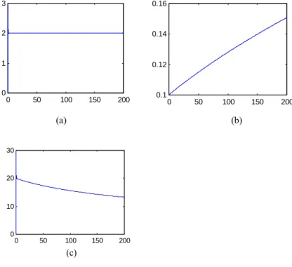
(a) (b)

(c)

Figure 6.3 Simulation results

The local control system performance can be improved by adding a first- or second-order reference filter [2], [6]. This is the way the control structure obtains the features specific to control structures with 2 DOF controllers.

For to test the method, a theoretical application closely connected to practice was considered. The non-linear Simulink model of the plant is presented in Appendix 1. Three PI controllers were calculated and the change of the controllers during the plant operating was based on a very simple fuzzy selection rule. The problem of bump-less transfer from one local crisp controller to another is solved in a crisp manner.

0 50 100 150 200

0 1 2 3

0 50 100 150 200

0.1 0.12 0.14 0.16

0 50 100 150 200

0 10 20 30

Some simulation results are presented in figure 6.3: (a) the change of the linear speed, v(t); (b) the change of the radius changing r(t); (c) the change of the angular speed, ω(t).

The results can be accepted as good and confirm the possibilitie of use Takagi- Sugeno fuzzy models to represent a TISO LTV as models of the controlled plant.

Conclusions

The paper presents continuous-time development solutions for electrical drives with variable inertia. The tuning relations are deduced for classical but generally accepted benchmark type plant models.

The presented TS fuzzy models dedicated to TISO LTV systems are suitable for control structures where the plant mathematical model linearization offers local linear models.

A stability test algorithm for the fuzzy control systems modeled by TS fuzzy models based on Lyapunov stability theory is presented. The main limitation of the stability analysis algorithm concerns its computational complexity.

The models and the stability analysis algorithm can be used in the development of conventional but also of TS fuzzy controllers based on the parallel distributed compensation with severalapplications. One real-world application can be in the area of electrical drives with variable inertia, where the development of the local controllers can be performed in terms of the ESO-m or 2E-SO-m.

The simulated application is regarded to a VIDS where the reference input must be correlated with the modification of working roll radius.

References

[1] Åström, K. J. and T. Hägglund: PID Controllers Theory: Design and Tuning, Instrument Society of America, Research Triangle Park, 1995 [2] Preitl, St. and R.-E. Precup, An extension of tuning Relations after

symmetrical optimum method for PI and PID controllers, Automatica, Elsevier Science, vol. 35, pp. 1731 – 1736, 1999

[3] Preitl, Zsuzsa, Controller development by algebraic methods. Analysis and Matlab-Simulink programs (in romanian). Master thesis, “Politehnica”

University of Timişoara, Romania, 2003

[4] Precup, R.-E. and St. Preitl, Development of Some Fuzzy Controllers with Non-homogenous Dynamics with Respect to the Input Channels Meant for a Class of Systems, Proceedings of ECCC-1999, (e-format) Karlsruhe, Germany

[5] Preitl, St., R.-E. Precup, Zsuzsa Preitl, Two Degree of Freedom Fuzzy Controllers: Structure and Development, Proceedings of the “In

Memoriam John von Neumann” Symposium, December, 2003, ISBN 963- 7154-21-3, pp. 49 – 60, Budapest, Hungary

[6] Preitl, Zsuzsa, PI and PID Controller Tuning Method for a Class of Systems, SACCS 20017^th International Symposium on Automatic Control and Computer Science, October 2001, Iasi, Romania (e-format)

[7] Preitl St. and R.-E. Precup, On the Fuzzy Control of a Class of Linear Time-Varying Systems, A&QT-R 2004, IEEE-TTC- Conference on Automation, Quality and Testing, Robotics, May 13–15, 2004, Cluj- Napoca, Romania

[8] Kóczy, L. T., Fuzzy If-Then Rule Models and Their Transformation into One Another. IEEE Trans. on SMC – part A, 26, (1996) 621-637

[9] H. O. Wang, K. Tanaka and M. F. Griffin, An Approach to Fuzzy Control of Nonlinear Systems: Stability and Design Issues, IEEE Transactions on Fuzzy Systems, (1996), vol. 4, pp. 14 – 23

[10] M. Johansson and A. Rantzer, Computation of Piecewise Quadratic Lyapunov Functions for Hybrid Systems, IEEE Transactions on Automatic Control, (1998), vol. 43, pp. 555 – 559

[11] M. Johansson, A. Rantzer and K. -E. Arzen, Piecewise Quadratic Stability of Fuzzy Systems, IEEE Transactions on Fuzzy Systems, (1999), vol. 7, pp. 713 – 722

[12] St. Preitl and R.-E. Precup. “PI controller design for speed control of DC drives with variable moment of inertia”. Bul.St. U.P.T., Trans. AC&CS.

Timisoara, Vol. 42(56), pp. 97 – 105. 1997

[13] St. Preitl, R.-E. Precup, On the Fuzzy Control of a Class of Linear Time- Varying Systems, AQTR 2004 (THETA 14), IEEE-TTTC- Conference on Automation, Quality and Testing, Robotics May, 2004, Cluj-Napoca, Romania

Appendix 1. The non-linear Simulink model of the plant

U a U c

i a

w (t )

r (t ) w (t ) o m e g a ( w (t ) )

o m e g a ( w (t ) ) o m e g a ( w (t ) )

r (t ) * w (t )

r (t ) * w (t ) r (t ) * r (t ) * w (t )

r (t ) r (t ) * r (t ) * w (t ) J i n f a s (t )

J s i s t (t )

r (t ) a * f h (t )

r (t ) r (t )

r 0 r 0

-K - a * h / (2 * p i ) a

a V s

V _ l i n i a r U a

w T o W o r k s p a c e 1

t T o W o r k s p a c e

S u m 4

S u m 3 S u m 2

S u m 1

S u m

S c o p e 3

S c o p e 2 S c o p e 1

S c o p e -K -

R a

P r o d u c t 5

P r o d u c t 4

P r o d u c t 3

P r o d u c t 2

P r o d 1 P r o d

-K - K m -K -

K e e

K e K e

-K - K c e

J p a r t J t g o l + J t r a n s f + J m

1 s I n t e g r a l w 1 1

s I n t e g r a l w 1

L a . s I n t e g r a l i a

1 s I n t e g r a l f h

-K - G a i n 1

-K - G a i n C l o c k

-K - C * a C

C