Obuda University ´
Doctoral Dissertation
Intelligent Decision Models
Author:
OrsolyaCsisz´ar
Supervisors:
Prof. Dr. J´anos Fodor Prof. Dr. R´obert Full´er
2015
ii Final Examination Committee:
Public Defence Committee:
Date of Public Thesis Defence:
Declaration of Authorship
I, Orsolya Csisz´ar, declare that this thesis titled, ’Intelligent Decision Models’ and the work presented in it are my own. I confirm that:
This work was done wholly or mainly while in candidature for a research degree at this University.
Where any part of this thesis has previously been submitted for a degree or any other qualification at this University or any other institution, this has been clearly stated.
Where I have consulted the published work of others, this is always clearly at- tributed.
Where I have quoted from the work of others, the source is always given. With the exception of such quotations, this thesis is entirely my own work.
I have acknowledged all main sources of help.
Signed:
Date:
i
”To keep your balance, you must keep moving.”
Albert Einstein
OBUDA UNIVERSITY´
Abstract
Doctoral School of Applied Informatics and Applied Mathematics
Doctor of Philosophy Intelligent Decision Models
by Orsolya Csisz´ar
This thesis is concerned with the development of intelligent decision models from a theoretical point of view. It covers two main topics: in chapters2-3, two special types of aggregation functions are studied, while in chapters 4-6, the so-called general nilpotent operator system is introduced and examined.
Chapter 1 gives an introduction to the topic of aggregation functions and intelligent decision modeling. The basic preliminaries are also given here.
In Chapter2, the properties of a new construction method of aggregation functions from two given ones, called threshold construction, are discussed. This class of non-symmetric functions provides a generalization of t-norms and t-conorms by partitioning the unit interval with respect to only one variable. In fuzzy modeling framework, the relationship of the input and the output can be modeled by splitting the input into fuzzy regions for which we can describe the output in different ways. In several applications, the roles of the inputs are not symmetric, which indicates the use of the examined construction.
The results of this chapter can be found in Csisz´ar and Fodor, [19].
Chapter 3 presents new construction methods of uninorms with fixed values along the borders. Sufficient and necessary conditions are presented. The results of this chapter can be found in Csisz´ar and Fodor, [20].
In Chapter4, the concept of a nilpotent connective system is introduced. It is shown that a consistent logical system generated by nilpotent operators is not necessarily isomorphic to Lukasiewicz-logic, which means that nilpotent logical systems are wider than we have thought earlier. Using more than one generator functions, three naturally derived negations are examined. It is shown that the coincidence of the three negations leads back to a system which is isomorphic to Lukasiewicz-logic. Consistent nilpotent logical structures with three different negations are also provided. The results of this chapter can be found in Dombi and Csisz´ar, [27].
In Chapter5, implication operators in bounded systems are deeply examined. Both R- and S-implications with respect to the three naturally derived negations of the bounded system are considered. It is shown that these implications never coincide in a bounded system, as the condition of coincidence is equivalent to the coincidence of the negations, which would lead to Lukasiewicz logic. The formulae and the basic properties of four different types of implications are given, two of which fulfill all the basic properties generally required for implications. The results of this chapter can be found in Dombi and Csisz´ar, [28].
Chapter6gives a detailed discussion of equivalence operators in bounded systems. Three different types of operators are studied. The paradox of the equivalence relation is solved by aggregating the implication-based equivalence and its dual operator. It is shown that
the aggregated equivalence has preferable properties such as associativity and threshold transitivity. The results of this chapter can be found in Dombi and Csisz´ar, [29].
The final Chapter 7 summarizes the main results and suggests some future research directions that could provide the next steps along the path to a practical and widely applicable system.
Acknowledgements
I am very grateful to Prof. Dr. J´anos Fodor and Prof. Dr. R´obert Full´er for their guid- ance, ideas and inspiration. Special thanks to Prof. Dr. J´ozsef Dombi for the fruitful collaboration, insight and many useful discussions. I would like to thank Dr. Anna Gy¨orgy for her strong support and for all of her advice. I am also grateful to the Lead- ership of the Doctoral School, to Prof. Dr. Aur´el Gal´antai and Prof. Dr. L´aszl´o Horv´ath for their encouragement and assistance. Finally, I would like to thank my family for their love and support which enabled me to complete this doctorate.
vi
Contents
Declaration of Authorship i
Abstract iii
Acknowledgements vi
Contents vii
List of Figures ix
List of Tables x
Abbreviations xi
Symbols xii
1 Introduction 1
1.1 Aggregation and decision . . . 1
1.2 Basic preliminaries . . . 3
1.2.1 Negations . . . 3
1.2.2 Triangular norms and conorms . . . 4
2 Threshold Construction of Aggregation Functions 8 2.1 Motivation and scope . . . 8
2.2 Properties . . . 9
2.3 Symmetrization . . . 10
2.4 Overview . . . 14
3 Uninorms with Fixed Values along Their Borders 15 3.1 Motivation and scope . . . 15
3.2 Results. . . 16
3.3 Overview . . . 27
4 The General Nilpotent Operator System 29 4.1 Motivation and scope . . . 29
4.2 Characterization of strict negation operators. . . 30 vii
Contents viii
4.3 Nilpotent connective systems . . . 32
4.3.1 Structural properties of connective systems . . . 34
4.3.1.1 Classification property. . . 35
4.3.1.2 The De Morgan law . . . 36
4.3.2 Consistent connective systems. . . 41
4.3.2.1 Bounded systems . . . 43
4.4 Overview . . . 47
5 Implication Operators in Bounded Systems 49 5.1 Motivation and scope . . . 49
5.2 Preliminaries . . . 50
5.3 R-implications in bounded systems . . . 52
5.4 S-implications in bounded systems . . . 55
5.4.1 Properties ofiSn, iSd and iSc . . . 56
5.4.2 S-implications and the ordering property. . . 57
5.5 Comparison of implications in bounded systems . . . 59
5.6 Min and Max operators in nilpotent connective systems . . . 60
5.7 Overview . . . 60
6 Equivalence Operators in Bounded Systems 64 6.1 Motivation and scope . . . 64
6.2 Preliminaries . . . 66
6.3 Equivalences in bounded systems . . . 67
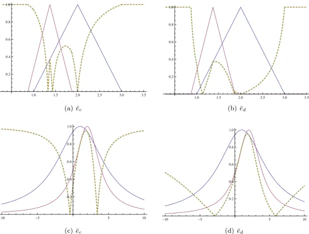
6.3.1 Properties ofec(x, y) anded(x, y) . . . 68
6.4 Dual equivalences . . . 71
6.4.1 Properties of ¯ed and ¯ec . . . 72
6.5 Arithmetic mean operators in bounded systems . . . 74
6.6 Aggregated equivalences . . . 75
6.6.1 Properties of the aggregated equivalence operator. . . 77
6.7 Applications. . . 81
6.8 Overview . . . 81
7 Main Results and Further Work 85
A Tables 88
Bibliography 92
List of Figures
1.1 Continuous negations with differentν∗ values . . . 4
2.1 Special types of A<T ,a,S>(x, y) . . . 9
2.2 Special types of B<T ,a,S>(x, y) . . . 11
2.3 Special types of C<T ,a,S>(x, y) and D<T ,a,S>(x, y) . . . 12
3.1 U1 and U2 . . . 19
3.2 U3 and U4 . . . 22
3.3 U5 . . . 22
3.4 U50 and U500 . . . 24
3.5 U6 . . . 25
3.6 U60 and U600 . . . 26
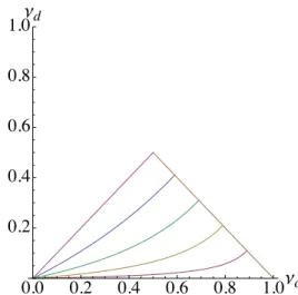
4.1 nd(x)< n(x)< nc(x) for α= 2 . . . 44
4.2 The relationship betweenν,νc and νd in consistent rational systems . . . 46
4.3 Conjunctionc[x, y] and disjunctiond[x, y] . . . 48
5.1 ic andid implications for rational generators. . . 61
5.3 Sc-implications for rational generators . . . 62
5.2 Sn-implications for rational generators . . . 62
6.1 ec(x, y) anded(x, y) for rational generators . . . 68
6.2 e¯c(x, y) and ¯ed with rational generators . . . 72
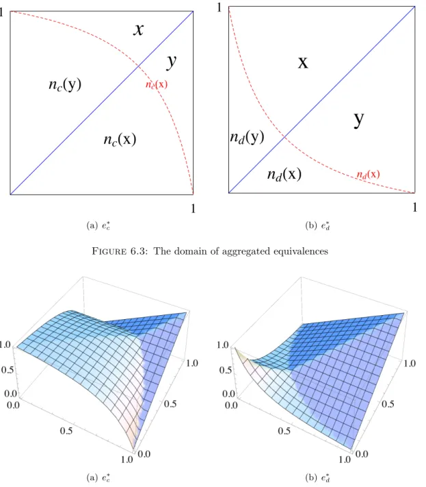
6.3 The domain of aggregated equivalences. . . 77
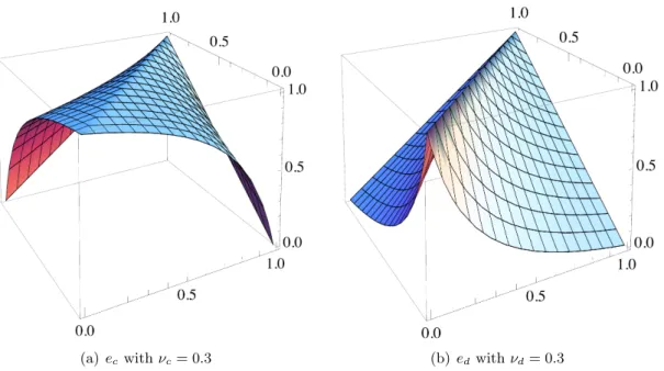
6.4 Aggregated equivalences with rational generators with ν= 0.3. . . 77
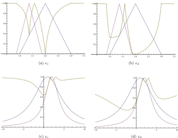
6.5 Pointwise equivalence of fuzzy numbers with rational generators (νc = νd= 0.3). . . 82
6.6 Pointwise dual equivalence of fuzzy numbers with rational generators (νc=νd= 0.3) . . . 83
6.7 Pointwise aggregated equivalence of triangular fuzzy numbers with ratio- nal generators (ν = 0.6) . . . 84
ix
List of Tables
A.1 Power functions as normalized generators . . . 88
A.2 Power functions as normalized generators – logical connectives . . . 88
A.3 Exponential functions as normalized generators . . . 89
A.4 Rational functions as normalized generators . . . 89
A.5 Rational functions as normalized generators – 3 negations . . . 89
A.6 Mixed types of normalized generator functions . . . 90
A.7 Properties of implications in bounded systems . . . 90
A.8 The main properties of equivalence operators . . . 91
x
Abbreviations
BC BoundaryCondition LC Law of Contraposition DF Dominance of Falsity DT Dominance of Truth EP Exchange Principle FA First PlaceAntitonicity IP Identity Principle
LN LeftNeutrality Property OP Ordering Property SI Second PlaceIsotonicity SN Strong Negation Property
xi
Symbols
c(x, y) conjunction d(x, y) disjunction e neutral element e(x, y) equivalence
ec(x, y) equivalence given by 6.7 ed(x, y) equivalence given by 6.7
¯
ec(x, y) dual equivalence given by6.15
¯
ed(x, y) dual equivalence given by6.15 e∗c(x, y) aggregated equivalence given by6.23 e∗d(x, y) aggregated equivalence given by6.23
fc(x) normalized additive generator function of a conjunctionc fd(x) normalized additive generator function of a disjunction d fn(x) generator function of a negationn
i(x, y) implication
ic(x, y) implication given by 5.5 id(x, y) implication given by 5.5 iR(x, y) residual implication iS(x, y) S-implication
mαc(x, y) weighted arithmetic mean operator given by6.21 mαc(x, y) weighted arithmetic mean operator given by6.21 n(x) negation
nc(x) negation generated by fc nd(x) negation generated by fd
S t-conorm
SD drastic sum
xii
Symbols xiii SL Lukasiewicz t-conorm
SM maximum
SP probabilistic sum
s(x) additive generator function of a t-conorm
T t-norm
TD drastic product TL Lukasiewicz t-norm
TM minimum
TP product
t(x) additive generator function of a t-norm
U uninorm
Umin uninorm given by3.1 Umax uninorm given by3.2 ν neutral value of a negation
νc neutral value of the negation generated byfc νd neutral value of the negation generated byfd [ ] cutting function given by 1.9
Dedicated to %
xiv
Chapter 1
Introduction
1.1 Aggregation and decision
Aggregation is the process of combining several numerical values into a single represen- tative one. The function, which performs this process is called an aggregation function.
Despite the simplicity of this definition, the size of the field of its applications is in- credibly huge: applied mathematics (e.g. probability theory, statistics, decision theory), computer sciences (e.g. artificial intelligence, operation research, pattern recognition and image processing), economics and finance, multicriteria decision aid, etc (see e.g.
[10], [43]).
If we think of the arithmetic mean, we can see that the history of aggregation is as old as mathematics itself. However, it was only in the last decades, when the rapid development of the above mentioned fields (mainly due to the arrival of computers) made it necessary to establish a sound theoretic basis for aggregation. The problem of data fusion, synthesis of information or aggregating criteria to form overall decision is of considerable importance in many fields of human knowledge. Due to the fact that data is obtained in an easier way, this field is of increasing interest.
One of the most prominent group of applications of aggregation functions comes from decision theory. Making decisions often leads to aggregating preferences or scores on a given set of alternatives, the preferences being obtained from several decision makers, experts, voters or representing different points of view, criteria, objectives. This concerns decision under multiple criteria or multiple attributes, multiperson decision making and multiobjective optimization [38].
The main factor in determining the structure of the needed aggregation function is the relationship between the criteria. At one extreme there is the case in which we desire
1
Chapter 1. Introduction 2 all the criteria to be satisfied. At the other extreme is the situation in which we want the satisfaction of any of the criteria. These two extreme cases lead to the use of ”and”
and ”or” operators to combine the criteria functions. A decision can be interpreted as the intersection of fuzzy sets, usually computed by applying a t-norm based operator, when there is no compensation between low and high degrees of membership. If it is interpreted as the union of fuzzy sets, represented by a t-conorm based operator, full compensation is assumed. However, it is obvious that no managerial decision represents any of these extreme situations.
As it is well-known, uninorms generalize both t-norms and t-conorms as they allow a neutral element anywhere in the unit interval. In the first part of the thesis (sections 2 and 3), results on further constructions of continuous aggregation functions are pre- sented.
Another outstanding application of aggregation functions comes from artificial intelli- gence, fuzzy logic [34]. Pattern recognition and classification, as well as image analysis are typical examples. According to Aristotle, in mathematics it was originally assumed that ”the same thing cannot at the same time both belong and not belong to the same object and in the same respect. [...] Of any object, one thing must be either asserted or denied.” The idea of many-valued logic was initiated by Jan Lukasiewicz around 1920. ”Logic changes from its very foundations if we assume that in addition to truth and falsehood there is also some third logical value or several such values” [50]. Many- valued logic was for several decades considered as a purely theoretical topic. It was the introduction of fuzzy sets by Zadeh in 1965 [82], which opened the way to fuzzy logics.
Aggregation functions are inevitably used in fuzzy logic, as a generalization of logical connectives. In artificial intelligence, these techniques are mainly used when a system has to make a decision. It is possible that the system has not only a single criteria for each alternative, but several ones. This case corresponds to a multicriteria decision-making problem. Furthermore, if a system needs a good representation of an environment, it needs the knowledge supplied by information sources in order to be reliable. However, the information supplied by a single information source (by a single expert or sensor) is often not reliable enough. That is why the information provided from several sensors (or experts) should be combined to improve data reliability and accuracy and also to include some features that are impossible to perceive with individual sensors.
One of the most significant problems of fuzzy set theory is the proper choice of set- theoretic operations [68, 77]. The class of nilpotent t-norms has preferable properties which make them more usable in building up logical structures. Among these properties are the fulfillment of the law of contradiction and the excluded middle, or the coincidence of the residual and the S-implication [33, 74]. Due to the fact that all continuous
Chapter 1. Introduction 3 Archimedean (i.e. representable) nilpotent t-norms are isomorphic to the Lukasiewicz t-norm [43] [50], the previously studied nilpotent systems were all isomorphic to the well-known Lukasiewicz-logic.
In the second part of the thesis (sections4,5and 6), logical systems, more specifically, nilpotent logical systems are in consideration. It is shown that a consistent logical system generated by nilpotent operators is not necessarily isomorphic to Lukasiewicz- logic. This new type of nilpotent logical systems is called a bounded system, which has the advantage of three naturally derived negations. Implication and equivalence operators in bounded systems are deeply examined and a wide range of examples is also presented.
1.2 Basic preliminaries
First, I recall some basic notations and results regarding negation operators, t-norms and t-conorms that will be useful in the sequel.
1.2.1 Negations
Definition 1.1. A unary operation n : [0,1] → [0,1] is called a negation if it is non- increasing and compatible with classical logic, i.e. n(0) = 1 andn(1) = 0.
A negation is strict if it is also strictly decreasing and continuous.
A negation is strong if it is also involutive, i.e. n(n(x)) =x.
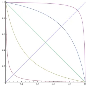
Due to the continuity and strict monotonicity ofn, for continuous negations there always exists someν∗, for whichn(ν∗) =ν∗ holds. ν∗ is called theneutral value of the negation and the notation nν∗ stands for a negation operator with neutral value ν∗. In the literature ν∗ is often denoted by e. In Figure 1.1 we can see some negations with different ν∗ values.
Drastic negations [78] are the so-called intuitionistic and dual intuitionistic negations (denoted by n0 and n1 respectively):
n0(x) =
( 1 if x= 0
0 if x >0 and n1(x) =
( 1 if x <1 0 if x= 1
These drastic negations are neither continuous nor strictly decreasing, therefore they are not strict negations, but we can get them as limits of strict negations.
Chapter 1. Introduction 4
0.2 0.4 0.6 0.8 1.0
0.2 0.4 0.6 0.8 1.0
Figure 1.1: Continuous negations with different ν∗ values
Definition 1.2. A continuous, strictly increasing functionϕ: [a, b]→[a, b] with bound- ary conditions ϕ(a) =a, ϕ(b) =b is called an automorphism of [a, b].
The well-known representation theorem was obtained by Trillas.
Proposition 1.3. (Trillas, [73]) n is a strong negation if and only if n(x) =fn−1(1−fn(x)),
where fn: [0,1]→[0,1] is an automorphism of [0,1].
Remark 1.4. This result also means thatnis a strong negation iff n(x) =fn−1 n0(fn(x))
(1.1) where fn, called the generator function of n,fn : [0; 1]→ [0; 1] is a strictly monotone, continuous function withfn(0) = 0 andfn(1) = 1 and n0 is a strong negation.
Example 1.1. For fn(x) =x2 andn0(x) = 1−x1+x we get n(x) =
q1−x2 1+x2. 1.2.2 Triangular norms and conorms
A triangular norm (t-norm for short)T is a binary operation on the closed unit interval [0,1] such that ([0,1], T) is an abelian semigroup with neutral element 1 which is totally ordered, i.e., for all x1,x2, y1,y2∈[0,1] withx1≤x2 and y1≤y2 we have T(x1, y1)≤ T(x2, y2), where ≤is the natural order on [0,1].
Chapter 1. Introduction 5 Standard examples of t-norms are the minimum TM, the product TP, the Lukasiewicz t-norm TL given by TL(x, y) = max(x+y−1,0), and the drastic product TD with TD(1, x) = TD(x,1) = x, and TD(x, y) = 0 otherwise. Clearly, TM and TD are the greatest and smallest t-norm, respectively, i.e., for each t-normT we haveTD≤T ≤TM. A triangular conorm (t-conorm for short) S is a binary operation on the closed unit interval [0,1] such that ([0,1], S) is an abelian semigroup with neutral element 0 which is totally ordered. Standard examples of t-conorms are the maximumSM, the probabilistic sumSP, the Lukasiewicz t-conormSLgiven bySL(x, y) = min(x+y,1), and the drastic sum SD with SD(0, x) = SD(x,0) = x, and SD(x, y) = 1 otherwise. Clearly, SM and SD are the smallest and greatest t-conorm, respectively, i.e., for each t-cnormSwe have SM≤S ≤SD.
A continuous t-norm T is said to beArchimedean ifT(x, x)< xholds for allx∈(0,1). A continuous Archimedean T is calledstrict ifT is strictly monotone; i.e. T(x, y)< T(x, z) whenever x ∈ (0,1] and y < z , and nilpotent if there exist x, y ∈ (0,1) such that T(x, y) = 0.
From the duality between t-norms and t-conorms, we can easily derive the following properties. A continuous t-conorm S is said to be Archimedean if S(x, x) > x holds for every x, y ∈ (0,1). A continuous Archimedean S is called strict if S is strictly monotone; i.e. S(x, y) < S(x, z) whenever x ∈ [0,1) and y < z, and nilpotent if there exist x, y ∈ (0,1) such that S(x, y) = 1. A t-norm is said to be positive if x, y > 0 implies T(x, y)>0.
From the duality between t-norms and t-conorms we can easily get the following prop- erties as well. A continuous t-conorm S is said to be Archimedean if S(x, x)> x holds for every x, y ∈ (0,1), strict if S is strictly monotone i.e. S(x, y) < S(x, z) whenever x∈[0,1) and y < z, and nilpotent if there existx, y∈(0,1) such that S(x, y) = 1.
Proposition 1.5. (Baczy´nski, [7], Ling, [53]) A functionT : [0,1]2 →[0,1]is a contin- uous Archimedean t-norm iff it has a continuous additive generator, i.e. there exists a continuous strictly decreasing functiont: [0,1]→[0,∞]witht(1) = 0, which is uniquely determined up to a positive multiplicative constant, such that
T(x, y) =t−1(min(t(x) +t(y), t(0)), x, y∈[0,1]. (1.2) Proposition 1.6. (Baczy´nski, [7], Ling, [53]) A functionS: [0,1]2 →[0,1]is a contin- uous Archimedean t-conorm iff it has a continuous additive generator, i.e. there exists a continuous strictly increasing functions: [0,1]→[0,∞]withs(0) = 0, which is uniquely
Chapter 1. Introduction 6 determined up to a positive multiplicative constant, such that
S(x, y) =s−1(min(s(x) +s(y), s(1)), x, y∈[0,1]. (1.3) Proposition 1.7. [43]
A t-norm T is strict if and only ift(0) =∞ holds for each continuous additive generator t of T.
A t-norm T is nilpotent if and only if t(0) < ∞ holds for each continuous additive generator t of T.
A t-conorm S is strict if and only if s(1) =∞ holds for each continuous additive gener- ator s of S.
A t-conorm S is nilpotent if and only if s(1) < ∞ holds for each continuous additive generator s of S.
In both of the above mentioned Propositions 1.5 and 1.6 we can allow the generator functions to be strictly increasing or strictly decreasing, which will result in the fact that they will be determined up to a (not necessarily positive) multiplicative constant.
For an increasing generator function t of a t-conorm and similarly for a decreasing generator function s of a t-conorm, min in (1.2) and (1.3) has to be replaced by max.
In this case we will have t(0) = ±∞ and s(1) = ±∞ for strict norms and similarly, t(0)<∞or t(0)>−∞and s(1)<∞ or s(1)>−∞ for the nilpotent ones.
Proposition 1.8. [43] Let T be a continuous Archimedean t-norm.
If T is strict, then it is isomorphic to the product t-norm TP , i.e., there exists an automorphism of the unit interval φ such thatTφ=φ−1(T(φ(x), φ(y))) =TP.
If T is nilpotent, then it is isomorphic to the Lukasiewicz t-norm TL, i.e., there exists an automorphism of the unit intervalφ such that Tφ=φ−1(T(φ(x), φ(y))) =TL. From the definitions of t-norms and t-conorms it follows immediately that t-norms are conjunctive, while t-conorms are disjunctive aggregation functions. Therefore, they are widely used as conjunctions and disjunctions in multivalued logical structures.
The logical system based on the nilpotent Lukasiewicz t-norm as conjunction is called Lukasiewicz-logic [45,54,63].
The use of the so-called cutting function makes the formulae simpler.
Chapter 1. Introduction 7 Definition 1.9. (Sabo et al., [66], Dombi and Csisz´ar, [27]) Let us define the cutting operation [ ] by
[x] =
0 if x <0 x if 0≤x≤1 1 if 1< x
and let the notation [ ] also act as ’brackets’ when writing the argument of an operator, so that we can write f[x] instead off([x]).
Chapter 2
Threshold Construction of Aggregation Functions
2.1 Motivation and scope
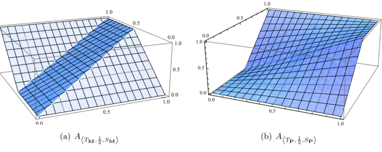
In 2012 Massanet and Torrens [58] introduced a new construction method of a fuzzy implication from two given ones. Now this idea is appropriately extended to construc- tions of continuous aggregation functions from a t-norm and a t-conorm, based on an adequate scaling on the second variable of the initial operators [19]. This construction can be usuful in fuzzy applications where the inputs have different semantic contents.
LetT be a t-norm,S be a t-conorm, anda∈(0,1). Let us define two binary operators as follows. Let
A<T ,a,S>(x, y) =
T(x,ya), if x∈[0,1], y∈[0, a]
S x,y−a1−a
, if x∈[0,1], y∈(a,1]
,
and
A<T ,a,S>(x, y) =A<T ,a,S>(y, x).
See Fig. 2.1.
8
Chapter 2. Threshold Construction of Aggregation Functions 9
0 0
0.5
1.0 0.0 0.5
1.0
0.0 0.5
1.0
(a)AhTM,12,SMi
0.0
0.5
1.0 0.0
0.5 1.0
0.0 0.5 1.0
(b) AhTP,12,SPi
Figure 2.1: Special types ofA<T ,a,S>(x, y)
2.2 Properties
In this section we examine the main properties, such as neutral or idempotent elements, associativity, of A<T ,a,S>(x, y) and A<T ,a,S>(x, y).
As it is easy to see,ais theright neutral elementofA<T ,a,S>(x, y), i.e.,A<T ,a,S>(x, a) = T(x,1) =x,for all x∈[0,1].Similarly, A<T ,a,S>(x,1) = 1 and A<T ,a,S>(x,0) = 0.
We can also see that ais anidempotent element ofA<T,a,S> and A<T,a,S>.
It can be shown that A<T ,a,S>(x, y) and A<T ,a,S>(x, y) are always monotone non- decreasing.
Due to the construction, both functionsA<T ,a,S>(x, y) and A<T ,a,S>(x, y) are continu- ous when T and S are continuous.
Since associativity is a key property of t-norms and t-conorms, it would be good to hand down some version of associativity to the constructions. A simple counterexample reveals that neitherA<T ,a,S>(x, y) norA<T ,a,S>(x, y) is associative for arbitraryT and S. Indeed, letT =TM,S =SM, and a= 12. Then we have
A<T ,a,S>
A<T,a,S>
2 3,2
3
,1 4
= 1
2 6=A<T ,a,S>
2
3, A<T ,a,S>
2 3,1
4
= 2 3. Thus, we study the following problem. Let T be a given t-norm. Does there exist a t-conormS such that A<T ,a,S> is associative?
To solve the functional equation of associativity, the following cases are to be examined:
1. y≤a, z≤a
Chapter 2. Threshold Construction of Aggregation Functions 10 2. y≤a, z > a
3. y > a, z≤a 4. y > a, z > a.
It can be shown that ifAis associative, thenT is necessarilya-migrative, i.e.,T(a, v) = av ∀v∈[0,1], see the definition and fundamental results about migrativity in [39].
In a similar way, we can conclude thatS(a, v) =a+ (1−a)v ∀v∈[0,1].
This means, that the a-migrativity is necessary but not sufficient condition of associa- tivity ofA. Indeed, for example whenT =TP, the constructedAwill not be associative.
Moreover, if we examine cases iii. and iv., we can see that A can never be associative on the whole unit square [0,1].
Studying the particular case when T =TP,SSP, and a= 12,we obtain
A<T
P,12,SP>(x, y) =
2xy, if x∈[0,1], y∈
0,12 2x+ 2y−2xy−1, if x∈[0,1], y∈ 12,1
.
It can easily be seen thatA<T
P,12,SP>(x, y) is not associative. Moreover,A<T
P,12,SP>(x, y) does not fulfill any of the associativity-like equations (see e.g. Grassmann, cyclic, Hossz´u in [56]), and it is not bisymmetric either.
2.3 Symmetrization
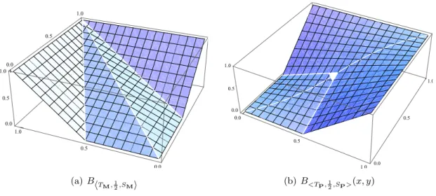
Since A<T,a,S>(x, y) and A<T ,a,S>(x, y) are obviously not symmetric, it is natural to study symmetrized versions of both functions. First we consider the following way of symmetrization of A<T ,a,S>, denoted by B<T ,a,S>:
B<T,a,S>(x, y) =A<T ,a,S>(min(x, y),max(x, y)).
See Fig. 2.2.
The monotonicity ofB<T ,a,S>(x, y) follows from the monotonicity ofA<T,a,S>(x, y).
The continuity of B<T ,a,S> follows from the continuity ofA<T ,a,S> and A<T ,a,S>. We can see thatB<T ,a,S>(x, y) is not associative for arbitrary T and S either.
Chapter 2. Threshold Construction of Aggregation Functions 11
0.0
0.5 1.0
0 0 0.5
1.0 0.0 0.5 1.0
(a)BhTM,12,SMi
0.0
0.5
1 0 0.0 0.5
1.0
0.0 0.5 1.0
(b) B<T
P,12,SP>(x, y)
Figure 2.2: Special types ofB<T ,a,S>(x, y)
Moreover,B<T
P,12,SP>(x, y) does not fulfil any of the associativity-like equations and it is not bisymmetric.
Let us study the particular case when T = TP, S = SP, and a = 12. In this case we obtain
B<T
P,12,SP>(x, y) =
2xy, if max(x, y)∈
0,12 2x+ 2y−2xy−1, if max(x, y)∈ 12,1 .
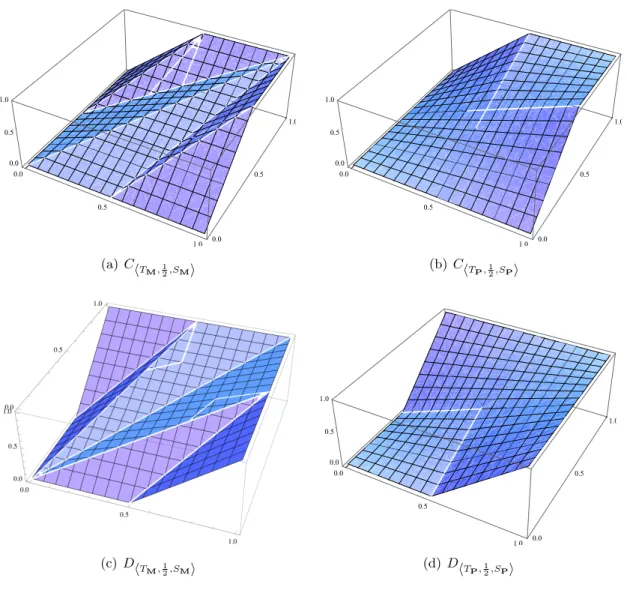
Now we define two further symmetrization ofA<T,a,S>, denoted byC<T,a,S>andD<T ,a,S>, as follows:
C<T ,a,S>(x, y) = min A<T ,a,S>(x, y), A<T,a,S>(x, y) and
D<T,a,S>(x, y) = max A<T,a,S>(x, y), A<T,a,S>(x, y) .
See Fig. 2.3. Both functions can be written in explicit forms, by applying the definitions of A<T ,a,S>:
C<T,a,S>(x, y) =
S
x,y−a1−a
, if x∈(a,1], y∈(a,1]
T x,ya
otherwise,
Chapter 2. Threshold Construction of Aggregation Functions 12
0.0
0.5
1 0 0.0 0.5
1.0
0.0 0.5 1.0
(a)ChTM,12,SMi
0.0
0.5
1 0 0.0 0.5
1.0
0.0 0.5 1.0
(b) ChTP,12,SPi
(c)DhTM,12,SMi
0.0
0.5
1 0 0.0 0.5
1.0
0.0 0.5 1.0
(d) DhTP,12,SPi
Figure 2.3: Special types ofC<T ,a,S>(x, y) andD<T ,a,S>(x, y)
and
D<T,a,S>(x, y) =
T x,ya
, if x∈[0, a], y∈[0, a]
S
x,y−a1−a
otherwise.
We can see thatC<T,a,S>(1, x) = 1 if x∈(a,1], and similarly,C<T,a,S>(0, x) = 0.
For D we obtain D<T ,a,S>(0, x) = 0 if x ≤a, and in this case D<T ,a,S>(0, x) = 0 also holds.
Clearly,C<T ,a,S>(x, y) and D<T ,a,S>(x, y) are monotone non-decreasing.
The continuity of C<T,a,S> and D<T ,a,S> follows from the continuity of A<T ,a,S> and A<T ,a,S>.
However, it can be shown thatC<T ,a,S>(x, y) is not associative.
Chapter 2. Threshold Construction of Aggregation Functions 13 Moreover,C<T
P,12,SP>(x, y) does not fulfil any of the associativity-like equations and it is not bisymmetric.
Studying the particular case when T =TP,S=SP, and a= 12, we obtain
C<TP,1
2,SP>(x, y) =
2xy, if x∈
0,12 , y∈
0,12
2x+ 2y−2xy−1, if x∈ 12,1
, y∈ 12,1
min (2xy,2x+ 2y−2xy−1), ifx∈ 0,12
, y∈ 12,1
min (2xy,2x+ 2y−2xy−1), ifx∈ 12,1 , y∈
0,12 , that is,
C<T
P,12,SP>(x, y) =
2x+ 2y−2xy−1, ifx∈ 12,1
, y∈ 12,1
2xy, otherwise.
Similarly, we have
D<T
P,12,SP>(x, y) =
2xy, if x∈
0,12 , y∈
0,12
2x+ 2y−2xy−1, if x∈ 12,1
, y∈ 12,1
max (2xy,2x+ 2y−2xy−1), ifx∈ 0,12
, y∈ 12,1
max (2xy,2x+ 2y−2xy−1), ifx∈ 12,1 , y∈
0,12 , i.e.
D<TP,1
2,SP>(x, y) =
2xy, if x∈
0,12 , y∈
0,12
2x+ 2y−2xy−1, otherwise.
Finally, using a representable uninorm U and its dual Ud instead of min and max in the process of symmetrization we can define another functions E<T ,a,S>(x, y) and F<T ,a,S>(x, y) as follows:
E<T ,a,S>(x, y) =U A<T ,a,S>(x, y), A<T,a,S>(x, y) and
F<T ,a,S>(x, y) =A<T,a,S>
U(x, y), Ud(x, y)
.
Chapter 2. Threshold Construction of Aggregation Functions 14 In the particular case when U is the so-called 3Π operator, ie., when
U(x, y) =
0 , if (x, y)∈ {(1,0),(0,1)}
xy
(1−x)(1−y) +xy , otherwise,
the symmetrized function F<T
P,12,SP>(x, y), does not fulfil any of the associativity-like equations and it is not bisymmetric either.
2.4 Overview
In this section, a new generation method of aggregation functions from two given ones, called threshold construction method, was examined. The most usual properties were investigated and the necessary conditions to ensure them were studied.
Thesis 1.1. The new type of aggregation function turned out to be monotonic and continuous, having a right-neutral and idempotent element. Three possible ways of symmetrizations are studied, two of them using min-max operators and the third using uninorms. After proving the lack of associativity in all cases, the bisymmetry and all the other associativity-like equations known from the literature are studied.
Chapter 3
Uninorms with Fixed Values along Their Borders
3.1 Motivation and scope
The concept of uninorms was introduced in 1996 by Yager and Rybalov [79], as a gener- alization of both t-norms and t-conorms (see also Dombi, [31]). Since their introduction, uninorms have been studied deeply by numerous authors from theoretical and also from application points of view. They turned out to be useful in many fields like expert systems [22], aggregation [80] and fuzzy integral [11, 49]. Idempotent uninorms were characterized in [21]. Recently, a characterization of the class of uninorms with strict underlying t-norm and t-conorm was presented in [41]. In [52] the authors showed that uninorms with nilpotent underlying t-norm and t-conorm belong to Umin or Umax. In this section some further construction methods of uninorms from given t-norms and t-conorms are discussed and sufficient and necessary conditions are presented.
The results of this section can be found in Csisz´ar and Fodor, [20].
Definition 3.1. A mapping U : [0,1]×[0,1]→[0,1] is a uninorm if it is commutative, associative, nondecreasing and there exists e ∈ [0,1] such that U(e, x) = x for all x∈[0,1].
The structure of uninorms was first examined by Fodor, Yager and Rybalov in [40].
First let us recall two classes of uninorms from [40] that play a key role in this section.
Proposition 3.2. Suppose that U is a uninorm with neutral element e∈]0,1[and both functions x→U(x,1)and x→U(x,0) (x∈[0,1]) are continuous except perhaps at the pointx=e. Then U is given by one of the following forms.
15
Chapter 3. Uninorms with Fixed Values along Their Border 16 1. If U(0,1) = 0then
U(x, y) =
eT xe,ye
, (x, y)∈[0, e]2; e+ (1−e)S
x−e 1−e,y−e1−e
, (x, y)∈[e,1]2;
min(x, y), otherwise.
(3.1)
2. If U(0,1) = 1then
U(x, y) =
eT xe,ye
, (x, y)∈[0, e]2; e+ (1−e)S
x−e 1−e,y−e1−e
, (x, y)∈[e,1]2;
max(x, y), otherwise.
(3.2)
The class of uninorms having form3.1is denoted byUmin, while the class with form3.2 is denoted by Umax.
3.2 Results
Proposition 3.3. (See also Li et al., [52].) Let T be a strict t-norm, S be a strict t-conorm and e∈]0,1[. The function
U1(x, y) =
eT xe,ye
, (x, y)∈[0, e]2; e+ (1−e)S
x−e 1−e,y−e1−e
, (x, y)∈[e,1]2;
1, x= 1 or y= 1;
min(x, y), otherwise.
(3.3)
is a uninorm with neutral element e (see Figure3.1).
Proof. To prove thatU1is a uninorm, we have to show that it is associative, commutative and that it has a neutral element e ∈ (0,1). Commutativity is obvious. From the properties of t-norms and t-conorms it follows immediately that e ∈(0,1) is a neutral element.
Note that U1 differs from Umin only at points where either x = 1 or y = 1. Since the associativity of Umin is already known from [40], we only need to concentrate on the border lines where at least one of the variables of U1 is 1.
To examine the associative equation
U1(x, U1(y, z)) =U1(U1(x, y), z), (3.4)
Chapter 3. Uninorms with Fixed Values along Their Border 17 we need to take the following possibilities into consideration:
1. Ifx= 1 or z= 1, then U1(x, U1(y, z)) = 1 =U1(U1(x, y), z).
2. If U1(y, z) = 1 or U1(x, y) = 1, then by using the strict monotonicity of S(x, y), we getx= 1 or y= 1.ThusU1(x, U1(y, z)) = 1 =U1(U1(x, y), z).
Remark 3.4. Note that the strict property of S cannot be omitted in Proposition 3.3 (i.e. the statement does not hold for arbitrary t-conorms). For a counterexample let us choose TP, SL,e= 0.3, x= 0.7,y= 0.8, andz= 0.In this caseU1(0.7, U1(0.8,0)) = 0, while U1(U1(0.7,0.8),0) = 1.
Proposition 3.5. (See also Theorem 4 in Li et al., [52].) U1 in (3.3) is a uninorm if and only if S is dual to a positive t-norm.
Proof. The condition is sufficient, since in this case the proof is similar to that of Propo- sition 3.3.
Now I show that it is also necessary.
Let us assume indirectly that there existx0, y0 6= 1,for whichU1(x0, y0) = 1.Obviously, x0, y0 > e. Let z0 < e, z0 6= 1 so thatU(y0, z0) 6= 1.In this case the right hand side of the associativity equation in (3.4) is trivially 1, while the left hand side isz0, which is a contradiction.
Proposition 3.6. Let T be a strict t-norm, S be a strict t-conorm and e∈]0,1[. The function
U2(x, y) =
eT xe,ye
, (x, y)∈[0, e]2; e+ (1−e)S
x−e 1−e,y−e1−e
, (x, y)∈[e,1]2;
1, x= 1, y 6= 0 or x6= 0, y= 1;
min(x, y), otherwise.
(3.5)
is a uninorm with neutral element e (see Figure3.1).
Proof. To prove thatU2is a uninorm, we have to show that it is associative, commutative and that it has a neutral element e ∈ (0,1). Commutativity is obvious. From the properties of t-norms and t-conorms it follows immediately that e ∈(0,1) is a neutral element.
Chapter 3. Uninorms with Fixed Values along Their Border 18 Note that U2 differs from U1 only at points (1,0) and (0,1). Since the associativity of U1 is already known (see Proposition 3.3), we only need to concentrate on the vertices of the unit square.
Since we examine the equation
U2(x, U2(y, z)) =U2(U2(x, y), z), (3.6) we need to take the following possibilities into consideration:
1. Forx= 0 or z= 0 the two sides of the associativity equation in (3.6) are trivially 0.
2. For x= 1 and U2(y, z) = 0 by using the strict monotonicity of T we obtain that eithery= 0 orz= 0. This obviously means that the two sides of the associativity equation in (3.6) are equally 0. The proof is similar forz= 1 and U2(x, y) = 0.
Remark 3.7. Note that the strict property cannot be omitted in the Proposition 3.6 (i.e. the statement does not hold for arbitrary t-norms and t-conorms). For a coun- terexample let us choose TL, SP, e = 0.3, x = 1, y = 0.1, and z = 0.1. In this case U2(1, U2(0.1,0.1)) = 0,whileU2(U2(1,0.1),0.1) = 1.
Proposition 3.8. (See also Theorem 5 in Li et al., [52].) U2 in (3.5) is a uninorm if and only if T(x, y) is a positive t-norm, andS(x, y) is dual to a positive t-norm.
Proof. This condition is sufficient, since in this case the proof is similar to that of Proposition3.6.
Now I show that it is also necessary. From the proof of Proposition 3.5 the necessity of the second condition is trivial. We only need to show that if U2(x, y) = 0 does not imply x = 0 or y = 0, then the associativity does not hold. Let us assume indirectly that there existy0, z0 6= 0,for whichU2(y0, z0) = 0.Obviously,y0, z0 < e.For x= 1 the left hand side of the associativity equation in (3.6) is trivially 0, while the left hand side is 1, which is a contradiction.
Chapter 3. Uninorms with Fixed Values along Their Border 19
min
min
S
T
1
1
e e
1 1
(a) U1
min
min
S
T
1
1
e e
1 1
(b) U2
Figure 3.1: U1 andU2
Proposition 3.9. (See also Li et al., [52].) Let T be a strict t-norm, S be a strict t-conorm and e∈]0,1[. The function
U3(x, y) =
eT xe,ye
, (x, y)∈[0, e]2; e+ (1−e)S
x−e 1−e,y−e1−e
, (x, y)∈[e,1]2;
0, x= 0 or y= 0;
max(x, y), otherwise.
(3.7)
is a uninorm with neutral element e (see Figure3.2).
Proof. To prove thatU3is a uninorm, we have to show that it is associative, commutative and that it has a neutral element e ∈ (0,1). Commutativity is obvious. From the properties of t-norms and t-conorms it follows immediately that e ∈(0,1) is a neutral element.
Note that U3 differs fromUmax only at points where either x = 0 or y = 0. Since the associativity of Umax(x, y) is already known from [40], we only need to concentrate on the border lines where at least one of the variables of U3 is 0.
To examine the associative equation
U3(x, U3(y, z)) =U3(U3(x, y), z), (3.8) we need to take the following possibilities into consideration:
Chapter 3. Uninorms with Fixed Values along Their Border 20 1. Ifx= 0 or z= 0, then U3(x, U3(y, z)) = 0 =U3(U3(x, y), z).
2. If U3(y, z) = 0 or U3(x, y) = 1, then by using the strict monotonicity of S(x, y), we getx= 0 or y= 0.ThusU3(x, U3(y, z)) = 0 =U3(U3(x, y), z).
Remark 3.10. Note that the strict property ofTcannot be omitted in Proposition3.9(i.e.
the statement does not hold for arbitrary t-norms). For a counterexample let us choose TL, SP, e= 0.3, x= 0.1, y = 0.1, and z = 0.8.In this case U3(0.1, U3(0.1,0.8)) = 0.8, while U3(U3(0.1,0.1),0.8) = 0.
Proposition 3.11. (See also Theorem 4 in Li et al., [52].) U3 in (3.7) is a uninorm if and only if T is a positive t-norm.
Proof. The condition is sufficient, since in this case the proof is similar to that of Propo- sition 3.9.
Now I show that it is also necessary.
Let us assume indirectly that there existx0, y0 6= 0,for whichU3(x0, y0) = 0.Obviously, x0, y0< e. Letz0 6= 0 so thatU3(y0, z0)6= 0.(It is easy to see that suchz0 always exists, since we can always chose z0 > e.) In this case the right hand side of the associativity equation in (3.8) is trivially 0, while the left hand side isz0, which is a contradiction.
Remark 3.12. Note that Proposition3.11 is dual to Proposition 3.5.
Proposition 3.13. (See also Li et al., [52].) Let T be a strict t-norm, S be a strict t-conorm and e∈]0,1[. The function
U4(x, y) =
eT xe,ye
, (x, y)∈[0, e]2; e+ (1−e)S
x−e 1−e,y−e1−e
, (x, y)∈[e,1]2;
0, x= 0, y 6= 1 or x6= 1, y= 0;
max(x, y), otherwise.
(3.9)
is a uninorm with neutral element e (see figure3.2).
Proof. To prove thatU4is a uninorm, we have to show that it is associative, commutative and that it has a neutral element e ∈ (0,1). Commutativity is obvious. From the properties of t-norms and t-conorms it follows immediately that e ∈(0,1) is a neutral element.
Chapter 3. Uninorms with Fixed Values along Their Border 21 Note that U4 differs from U3 only at points (1,0) and (0,1). Since the associativity of U3 is already known (see Proposition 3.9), we only need to concentrate on the vertices of the unit square.
Since we examine the equation
U4(x, U4(y, z)) =U4(U4(x, y), z), (3.10) we need to take the following possibilities into consideration:
1. Forx= 1 or z= 1 the two sides of the associativity equation in (3.6) are trivially 1.
2. For x= 0 and U4(y, z) = 1 by using the strict monotonicity of S(x, y) we obtain that either y = 1 or z = 1. This obviously means that the two sides of the associativity equation in (3.6) are equally 1. The proof is similar for z = 0 and U4(x, y) = 1.
Remark 3.14. Note that the strict property cannot be omitted in the Proposition 3.13 (i.e. the statement does not hold for arbitrary t-norms and t-conorms). For a coun- terexample let us choose TP, SL, e = 0.3, x = 0, y = 0.8, and z = 0.9 In this case U4(0, U4(0.8,0.9)) = 0,whileU4(U4(0,0.8),0.9) = 1.
Proposition 3.15. (See also Theorem 5 in Li et al., [52].) U4 in (3.9) is a uninorm if and only if T is a positive t-norm, andS is dual to a positive t-norm.
Proof. The condition is sufficient, since in this case the proof is similar to that of Propo- sition 3.13.
Now I show that it is also necessary. From the proof of Proposition3.11the necessity of the first condition is trivial. We only need to show that ifU4(x, y) = 1 does not imply x= 1 ory = 1, then the associativity does not hold. Let us assume indirectly that there existsy0, z0 6= 1,for which U4(y0, z0) = 1.Obviously,y0, z0> e. Forx= 0 the left hand side of the associativity equation in (3.10) is trivially 1, while the left hand side is 0, which is a contradiction.
Remark 3.16. Note that Proposition3.15 is dual to Proposition 3.8.
Chapter 3. Uninorms with Fixed Values along Their Border 22
max
max
S
T
0
0 e
e
1 1
(a) U3
max
max
S
T
0
0 e
e
1 1
(b) U4
Figure 3.2: U3 andU4
min
min
S
T
1
1
e a
e
a 1 1
(a)
min
min
S
T1 T2
1
1
e a e a
1 1
(b) Figure 3.3: U5
Let us now consider a function U5 such that
U5(x, y) =
eT xe,ye
, (x, y)∈[0, e]2; e+ (1−e)S
x−e 1−e,y−e1−e
, (x, y)∈[e,1]2;
1, x= 1and y ≥a or y = 1 and x≥a;
min(x, y), otherwise.
(3.11)
whereT is a t-norm,S is a t-conorm, e∈]0,1[, a∈]0, e[ (see Figure 3.3).
Chapter 3. Uninorms with Fixed Values along Their Border 23 Let us consider the conditions under whichU5 can be a uninorm. Suppose thatU5 is a uninorm with neutral element e.
Proposition 3.17. If U5 is a uninorm with neutral element e, then U5(a, a) =a.
Proof. From the conjunctive property of t-norms it follows immediately thatU5(a, a)≤ a. SupposeU5(a, a)< a. Then by the definition ofU5,U5(1, U5(a, a))<1.On the other hand, by assiociativity, U5(U5(1, a), a) =U5(1, a) = 1, a contradiction.
Corollary 3.18. IfU5 is a uninorm with neutral valuee, then T is an ordinal sum (see Figure3.3) of two t-norms, T1 and T2, i.e.
T(x, y) =
a·T1 xa,ya
if (x, y)∈[0, a]2 a+ (e−a)·T2
x−a e−a,y−ae−a
if (x, y)∈[a, e]2
min(x, y) otherwise
(3.12)
Corollary 3.19. U50 and U500 defined below are also uninorms (see Figure 3.4):
U50(x, y) =
eT2 x
e,ye
, (x, y)∈[0, e]2; e+ (1−e)S
x−e 1−e,y−e1−e
, (x, y)∈[e,1]2;
1, x= 1 or y= 1;
min(x, y), otherwise.
(3.13)
U500(x, y) =
eT1 x
e,ye
, (x, y)∈[0, e]2; e+ (1−e)S
x−e 1−e,y−e1−e
, (x, y)∈[e,1]2;
1, x= 1 or y= 1;
min(x, y), otherwise.
(3.14)
Corollary 3.20. From Proposition 3.3and Corollary 3.19 it follows immediately, that if U5 is a uninorm, then S must be dual to a positive t-norm.
Proposition 3.21. U5 is a uninorm if and only if S is dual to a positive t-norm.
Proof. The necessity of this condition is the statement of Corollary 3.20. Now I prove that is is also sufficient. Note that U5 differs from Umin only at points (x, y), where a≤x < e andy = 1,ora≤y < e andx= 1. Since the associativity of Umin is already known, we only need to concentrate on these regions.