Optimization-based analysis and control of complex networks with nonlinear dynamics
Komplex, nemlineáris dinamikájú hálózatok analízise és irányítása optimalizálási módszerekkel
János Rudan
A thesis submitted for the degree of Doctor of Philosophy
Pázmány Péter Catholic University Faculty of Information Technology and Bionics
Supervisors:
Prof. Gábor Szederkényi (PPCU FIT) Prof. Katalin M. Hangos (HAS SZTAKI)
Budapest, 2014.
Non est volentis, neque currentis, sed miserentis Dei
Acknowledgements
First of all, I would like to thank Prof. Katalin M. Hangosand Prof. Gábor Szederkényi for their continuous support, guidance and encouragement during my studies.
I would also like to thankZoltán Tuza for all the work we have done together through our student years.
I wish to express my gratitude to all my colleagues for their advice, and for discussing about my ideas: Dóra Bihary, Bence Borbély, Dr. Csercsik Dávid, Balázs Jákli, Csaba Józsa, György Lipták,István Reguly,Norbert Sárkány,Dr. András Horváth,Miklós Koller,Mihály Radványi, Gábor Tornai and Dr. Kristóf Iván. It was a pleasure for me to work with you. I also would like to thank Bart Kersbergen,Ton van den Boom andProf. Bart De Schutter for the opportunity of joint research. I am grateful to the Delft University of Technology for hosting me as guest researcher.
I owe sincere thankfulness to Dr. Judit Nyékyné Gaizler, Dr. Péter Szolgay and Dr.
Tamás Roska, and I could not have completed this work without the support of the Faculty of Information Technology and Bionics of Pázmány Péter Catholic University.
I am especially grateful to Csenge for all her patience and support.
Last but not least, I am very grateful to my mother and father and to my whole family who always supported me in all possible ways.
Part of the work has been supported by the grants K83440 and NF104706 of the Hungarian Research Fund.
Abstract
There are several types of dynamical systems that can be described as networks. It is also known, that graph-based system description is a powerful tool to represent networked system structures on different levels of abstraction.
As the focus of the research of networked systems shifted towards the large-scale networks constructed from real-life data, the importance of highly effective computational methods applicable for the analysis and control of these systems increased. Due to the rapid devel- opment of computer technology and the underlying computational and analytical methods, optimization methods became an important tool in system theory, applied also for the optimal control of complex, networked systems.
The work summarized in this thesis focuses on the application of centralized, but par- allelizable optimization-based methods in the analysis and control of networked systems having nonlinear dynamics. Two classes of networked systems are investigated because they come from basically different approaches of networked system description, while they can be handled with similar mathematical tools.
Firstly, new methods for the structural and dynamical analysis of kinetic reaction networks are proposed. With the help of the introduced algorithms, the search for different alternative realizations of dynamically equivalent or linearly conjugate reaction networks can be completed while considering dynamical and/or structural constraints. Moreover, most of the algorithms have polynomial time complexity enabling us to handle large scale, biologically relevant networks, too. Extensive simulations are completed to evaluate the performance and the correctness of the proposed methods.
Secondly, optimal rescheduling method for the control of railway networks in case of delayed operation is proposed. The presented controller is capable to generate new timetables for the network in order to minimize the sum of the train delays along the prediction horizon.
Moreover, with the help of the proposed framework the sensitivity of the railway network can be measured in case of single delays. Additionally, a new model formulation is introduced having an advantageous constraint structure, which gives the opportunity of the deeper analysis of the dependencies between events and control actions in the network. The proposed methods are tested on the model of the Dutch railway network.
Összefoglalás
A hálózatos formában történő reprezentáció gyakran hasznos eszköz bizonyos dinamikus rendszerek működésének megértésében és leírásában. Ismert tény, hogy a gráf alapú leírás hatékony eszköz a hálózatos struktúrájú rendszerek különböző absztrakciós szinten történő leírására.
Ahogy a hálózatos struktúrájú rendszerek kutatásának fókusza az adat-alapú, nagy méretű hálózatok vizsgálata felé tolódik, úgy nyernek egyre nagyobb teret az ilyen típusú rendszerek analízisére és irányítására alkalmazható, hatékony számítási módszerek. A számítógépes tech- nológiák és a segítségükkel alkalmazott számítási és analitikai megoldások gyors fejlődésének köszönhetően az optimalizációs módszerek igen fontos eszközzé váltak a rendszerelméletben, melyeket gyakran alkalmaznak a komplex, hálózatos rendszerek optimális irányítására is.
A jelen dolgozatban összefoglalt munka fókuszában a nagyméretű, nemlineáris dinamikával rendelkező hálózatos struktúrájú rendszerek centralizált, de párhuzamosítható optimalizálási módszereken alapuló analízise és irányítása áll. Két hálózatokon alapú modellosztályt vizs- gáltam, amelyek leírásai alapvetően más megfontolásokból származnak, ám mégis hasonló matematikai módszerekkel kezelhetők.
Egyrészről új módszereket adtam kinetikus reakcióhálózatok strukturális és dinamikus tulajdonságainak analízisére. A bemutatott módszerek segítségével dinamikusan ekvivalens ill.
lineárisan konjugált alternatív reakcióhálózatok határozhatók meg dinamikus és/vagy struk- turális korlátozások figyelembe vétele mellett. A javasolt algoritmusok legtöbbje polinomiális időbeli komplexitással rendelkezik, ami lehetővé teszi azt, hogy nagy méretű, biológiailag releváns hálózatokat kezeljünk segítségükkel. A bemutatott módszerek helyességét és teljesít- ményét kiterjedt szimulációkkal vizsgáltam.
Másrészről optimális újraütemezésen alapuló irányítási módszert javasoltam késéses esetek kezelésére vasúti hálózatokban. A bemutatott szabályzó új menetrendeket állít elő olyan módon, hogy a predikciós horizont mentén minimális legyen a vonatok késésének összege. Emellett a módszer lehetőséget ad a vasúti hálózat érzékenységének vizsgálatára vonatok egyedi késése esetén. Új, előnyös korlátozás-struktúrát mutató problémaalakot javasoltam, melynek segítségével a hálózatban történő események és a kontrollváltozók közötti kapcsolatok könnyen vizsgálhatók. A bemutatott módszereket a holland vasúti hálózat modelljén szimuláltam.
Contents
1 Introduction 6
1.1 Networks in system modeling . . . 7
1.2 Aim and structure of this thesis . . . 8
1.3 Optimization in system analysis and control . . . 9
1.4 Networks and dynamics . . . 10
1.5 Kinetic reaction networks as unified models of smooth nonlinear systems . . . 13
1.6 Transportation networks . . . 15
2 Basic tools and notations 16 2.1 Convex optimization . . . 16
2.2 Linear Programming . . . 17
2.2.1 Problem formulation . . . 18
2.2.2 Solution methods . . . 19
2.2.3 Comparison of solution methods . . . 21
2.3 Mixed Integer Linear Programming . . . 21
2.3.1 Problem formulation . . . 22
2.3.2 Solution methods . . . 22
3 Applying optimization methods to find kinetic reaction networks with preferred structural and dynamical properties 26 3.1 Kinetic Reaction Networks . . . 27
3.1.1 Describing a kinetic system as a KRN . . . 27
3.1.2 Dynamical equivalence and linear conjugacy of KRNs . . . 30
3.1.3 Known methods to compute dynamically equivalent KRNs . . . 34
3.1.4 Weak reversibility . . . 38
3.1.5 Known methods to compute dynamically equivalent, weakly reversible KRNs . . . 42
3.1.6 Mass conservation in KRNs . . . 43
3.2 Finding dynamically equivalent realizations with LP . . . 44
3.2.1 Finding sparse realizations . . . 44
3.2.2 Finding dense realizations . . . 45
3.2.3 Comparative study of the presented algorithms . . . 47
3.2.4 Possible parallelization of the proposed algorithms . . . 48
3.2.5 Finding sparse/dense realizations in case of large kinetic reaction networks 49 3.3 Finding dynamically equivalent weakly reversible realizations with LP . . . . 49
3.3.1 Introduction of new algorithms to compute weakly reversible realizations 50 3.3.2 Performance analysis of the different methods . . . 55
3.4 Finding dynamically equivalent realizations with mass conservation . . . 57
3.5 Summary . . . 60
4 Efficient scheduling of railway networks using optimization 62 4.1 Optimization-based control of railway networks to minimize total delays . . . 63
4.1.1 Basics of the model formulation . . . 63
4.1.2 Constraint set formulation . . . 65
4.1.3 MILP problem formulation . . . 68
4.1.4 Introducing delays into the model . . . 70
4.2 New solution methods of the railway scheduling problem to increase solution efficiency . . . 71
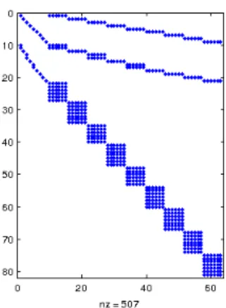
4.2.1 Track-based transformation of the problem matrix . . . 72
4.2.2 Transformation of individual constraints . . . 73
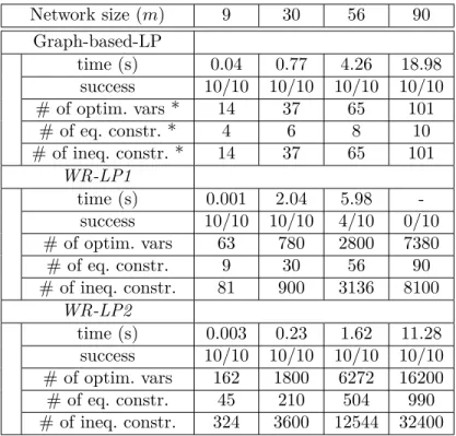
4.3 A case study . . . 79
4.3.1 Performance analysis of the proposed control technique . . . 82
4.3.2 Comparison of time consumption of solutions in case of different model formulations . . . 82
4.3.3 Sensitivity analysis based on single delays . . . 85
4.4 Summary . . . 87
5 Conclusions 89 5.1 New scientific contributions of the work (thesis points) . . . 89
5.2 Utilization of the presented results, further work . . . 91
The Author’s Publications 93 References 94 Appendix 104 A. List of abbreviations . . . 104
B. List of notations . . . 105 C. Procedural description of the transformation method presented in Sec. 4.2.2 106
Chapter 1
Introduction
Dynamical models have central role in several fields of science and technology. With them we can describe the operation of production processes, power generation systems, transportation networks and individual vehicles, agent-based systems etc. Besides models applied in traditional engineering fields, numerous biological processes and phenomena can also be understood and explained by creating their dynamical model. Dynamical modeling becomes necessary if the state of the investigated system, namely the quantities describing the properties of the system, evolves in time and/or space [96].
As a complex system we mean large-scale dynamical systems with complex structure containing nonlinearities. An important requirement in the modeling of complex systems is simplification: the model should most importantly describe only those phenomena and processes which have significant effect on the dynamics of the system. Using a dynamical model, the future behavior of the system can be predicted with respect to a given initial state, thus the analysis and simulation of the system is possible. These are crucial steps towards the controlling of the given system which is essential to achieve desired operation.
The understanding and targeted manipulation of these kind of models are the main topics of system and control theory.
In order to describe a large scale, complex system having many components proper structuring of the model should be applied [15]. A modular and clean model formulation helps to capture and understand the most important properties of the investigated system.
To accomplish this, a widely used and straightforward way is to separate the dynamics of the individual parts/elements and the connections between them leading to a description with networked structure. A deeply investigated and well known example of this phenomena is the theory of linear networks [42]. A more detailed review of the networked systems can be found in Sec. 1.1.
Nonlinearities in a system can be incorporated into the system model through several ways. Using continuous models, the simplest case is to introduce smooth nonlinearities optionally extended with discrete variables to describe switching-type events. In case of applying discrete models, the theory of discrete event systems [102, 7] is able to handle many
important phenomena.
From these theories, it is known, that we can classify dynamical models based on different points of view [91]. By determining the model class corresponding to the investigated system, we are able to determine the set of applicable methods and techniques for the analysis and control of the given system.
Because of the complex nature of many practically relevant control problems, the methods applicable for nonlinear systems with a networked structure are especially important, but they present challenges at the same time. This thesis focuses on the optimization-based solutions of the control problems related to complex systems having networked structure.
1.1 Networks in system modeling
There are several types of dynamical systems that can be described as networks. Supply chains, transportation and public transport networks, in-cell reaction systems, genetic reg- ulatory networks are some of the widely investigated systems having networked structure.
Basically, networks consist of two main elements: a set of nodes and a set of links connecting the nodes to each other. Both the nodes and the links can be static or dynamic elements, depending on the properties of the system described by the network [15].
Usually, to describe the structure of networks in a mathematical framework, graph theory is used where nodes and links in the network are corresponding to vertices and edges in the graph, respectively. The way, how graphs can describe dynamical systems can have multiple interpretation: e.g. in case of transportation networks a topographical layout of vertices and edges can be handful, representing junctions and sections of the network. Meanwhile, a more abstract, graph-based description of a system is also possible, e.g. in case of discrete event systems, where vertices are standing for the different states of the system while edges represent possible state transitions. As it can be seen from these examples the graph-based system description is a powerful tool to represent several system structures on different levels of abstraction.
If we investigate a static system a graph-based representation of the system can describe structural dependencies between the components of the system where both the vertices and edges are static or passive. If the dynamics is also incorporated into the system description, the following setup is usual. The vertices represent the individual components of the system, while the edges between them set constraints on the behavior of the dynamics. The quantitative properties of the constraints usually appear as edge weights in a weighted, directed graph.
The topic of combining several, individual dynamical systems into a complex, networked system is elaborated in the theory of interconnected subsystems in systems and control theory.
In [36] mathematical tools are provided to analyze the connectability of composite systems, which property ensures the controllability and observability of the complex system. The fact, that the controllability and observability of a networked system depends on the properties of
the linkages between the components leads to the concept of structural controllability and observability [78]. These ideas are further developed in [79] showing the crucial properties of a relatively small number of driver nodes while controlling the dynamics of a complex networked system.
The importance of the quality and quantity of the connections in the graph is emphasized by the research of the dynamics appearing in extreme large networks, such as social networks [14]. The statistical analysis of the behavior patterns in these kind of networks enables us to understand the significance of weak connections in social communities, the reordering patterns in such systems etc. As several databases became available containing data about large-scale networks, the techniques to analyze the data moved towards fractal-based description [113], graph-focused data mining techniques [66] and other improved techniques, which instead of analyzing the individual elements of the network, focus on the graph-theory based description of the representing structures.
The work summarized in this thesis focuses on the application of optimization-based methods in the analysis and control of networked systems. Two classes of networked systems are investigated because they come from basically different approaches of networked system description, while they can be handled with similar mathematical tools. In case of a reaction network, the model is translated into a network by describing the relations between the terms of the underlying differential equations as links between the nodes of a network that represent the elementary nonlinearities. In contrast with this, in transportation networks (in this particular case, in railway networks) both the nodes and the links are passive, they are only a topological mapping of the routes, junctions and/or stations. Nonlinearities are introduced into this model by the absolute values appearing in the basic system model. Both system classes are nonnegative [60], and can be handled as smooth nonlinear systems (by incorporating vehicle dynamics into the microscopic modeling of the system).
1.2 Aim and structure of this thesis
The aim of the present thesis is to develop optimization based methods applied to the analysis and control of specific, practically important dynamical systems having complex networked structure. By analyzing the structure of the original, networked system and the structure of the emerging optimization problem, problem-specific improvements are proposed to decrease the complexity of the computational tasks, thus they become applicable on large scale networks, too. Generally, these tasks are formulated as MILP problems, but in several cases, they can be simplified to Linear Programming (LP) tasks.
In this thesis, two different system classes are examined having networked structure:
kinetic reaction networks and railway networks. In both cases, we will use optimization- based techniques to solve problems in the field of system analysis and control. In case of reaction networks, structural (parameter-independent) system analysis and the computation
of alternative reaction networks will be completed using optimization based methods.
In case of the railway networks control actions are going to be computed for optimal rescheduling in order to minimize the sum of the delays of the trains. By applying optimization based control methods, our aim is to decrease the sensitivity of the railway network against small appearing delays and by reducing the delay propagation effect. To accomplish this, a model formulation is needed which enables us to simplify the analysis of the effect of the dispatching actions with respect to the individual delays of the trains. It is also desired, that formulated optimization problems should be solvable in a reasonable time, thus the possibility to handle large-scale networks with algorithms using them is present.
The structure of the thesis is the following. In Chapter 2 the basic notions and the mathematical tools are introduced, which serve as a basis of the methods presented in the further parts of this work. Chapter 3 introduces the Kinetic Reaction Networks in details, summarizes the results known from the literature and the corresponding results of the author.
In Chapter 4 the topic of railway networks are investigated, presenting the different model formulations, the proposed new methods and the simulation results. In Chapter 5 the main scientific contributions of the presented work are briefly summarized and the possible further developments are enumerated.
1.3 Optimization in system analysis and control
As it is detailed in [24], optimization problems play an important role in several fields of system theory. In particular, any controller design problem is in fact a constrained optimization problem with the control aim as loss function and the system model as a constraint.
Due to the rapid development of computer technology and the available computational and analytical methods, several new application area of optimization methods appeared in system theory. Two application domains have become particularly important: the computational methods themselves and those conceptual developments which make it possible to implement the developed methods in real-life applications (e.g. Model Predictive Control framework [53]). Considering the underlying computational methods, it can be said, that most of the formulated optimization problems can be traced back to mathematical programming problems which are able to handle cost functions and constraints on the variables.
With the help of the tools emerging from optimization several different tasks in system analysis and control can be solved: identification problems, parameter estimation tasks and control problems can also be formulated in such a framework [80]. Identification and parameter estimation form a closely inter-related set of problems where the application of optimization methods focuses on the computation of system parameters using the presented, usually noisy and limited measurement data [126]. Several methods applied in the control of dynamic systems can also be traced back to optimization: e.g. the method of Linear Matrix Inequalities [23] to design robust controllers, decentralized control [54] to deal with systems
incorporating multiple decision maker units, Linear-Quadratic (LQ) control problems [83] in classical control theory or state estimation [112].
Techniques applied in optimal control were further developed to the control of networked systems, where the entities of the system are connected to each other via links, altogether considered as a graph structure as it is detailed before. Optimization tasks are formulated from the coordinated control task of the entities in case of different connectivity properties [68], synthesis of complex process plants with a networked structure [50] satisfying different type of constraints and having objective functions with multiple components etc. Also, methods are developed to compute different properties and representations of a given system having networked structure, such as minimal representation, identifying key connections etc. One of the developed methods is capable of computing a maximal superstructure corresponding to a given process network in polynomial time [49] in a centralized way. From the computed superstructure, with the help of additionally applied constraints all possible solutions of the original problem can be extracted enabling us to analyze the properties of the solutions with high computational efficiency. As the focus of the research of networked systems shifted towards the large-scale networks constructed from real-life data, the importance of the highly effective computational methods applicable for the solution of optimization problems increased.
Problem formulation in an optimization framework has a great conceptual importance:
in case of a properly formulated problem its feasibility can be checked, meaning that the existence of at least one solution can be shown even if the underlying problem is hard to solve. The fact, that infeasibility (non-existence of a solution) can be explicitly detected has great importance both in theory and in application.
The aim of the present thesis is to investigate the analysis and control of complex nonlinear dynamical systems having networked structure using optimization-based techniques. This topic is examined through two problems, namely the structural and dynamical analysis of kinetic reaction networks and the dynamical rescheduling problem of railway networks. In case of both problems, we formulate the dynamical model of the corresponding networked system and the solutions of the examined tasks are derived to a mathematical optimization problem. In case of reaction networks a structural analysis has been completed and alternative realizations are computed, while in case of railway networks, the effect of delay propagation is reduced by applying optimal control actions in the schedule of the trains.
1.4 Networks and dynamics
The research of systems composed by a large number of interconnected dynamical units gained increased attention recently. The analysis and modeling of large scale coupled systems from the field of biology, chemistry, transportation, logistics, social sciences etc. became an important topic in science as the computational performance of the computer systems grows
and the detailed processing of huge amount of data is possible. This gives us the opportunity to shift our attention from the investigation of individual properties of small-scale networks towards the analysis of large scale systems with complex interconnection patterns, sometimes by focusing only on the statistical properties of the modeled system. Some important results about these topics are summarized in [89].
The two main issues while investigating a complex coupled system are the following:
firstly, to identify the structure of the connections between the actors of the system in order to describe the system with the help of phenomena known from classical network theory. Here the central task is to properly define the nodes in the network and the links in between them, which usually considered as vertices and edges in the graph corresponded to the network, respectively. Secondly, the type and behavior of the interactions should be identified with respect to the formulated structure. These can be described as the properties of the edges in the graph of the network. The obtained network models can be applied to analyze and if it is needed, to control the underlying dynamics. A detailed review of the possible model classes and their applications can be found in [19].
Among many others, complex networked systems can be classified based on the role of the nodes in the network. In one hand, there are model types where the nodes have active role in the dynamics of the network (they have some generalized computing task), and the network can be considered as a set of agents connected to each other as it is defined by the structure of the network. On the other hand there are models where nodes are only interconnecting elements in the network connecting different edges, but they do not have specific ”computational” tasks. These kind of models are similar to pipeline networks, where nodes are created at the junctions of pipe sections.
Let us shortly review some system classes that can be modeled with the previously introduced, agent-based network formulation.
Artificial neural networks are motivated by biological neural networks, and their aim was to create a computational method that has as strong learning capabilities as the biological neural networks have. The proposed perceptron model [106] is based on strong simplifications of the biological neurons but still tried to capture their main properties. The artificial neural network is defined as a set of processing nodes which have similar role than the cell body of neurons while weighted edges connect the processing nodes as the axons connect neurons. The connectivity pattern strongly influences the behavior of the network and some classical configuration of artificial networks emerged such as feed-forward networks and Hopfield-networks [64].
The phenomena of individual processing nodes connected by weighted edges further developed leading to the appearance of Cellular Neural Networks (CNN) [31]. CNNs are a general framework to build parallel processing units with nonlinear dynamics arranged topographically in a grid. The connections between the nodes are local: only neighboring processing units can communicate with each other, thus the behavior of the whole network
is characterized by the local connections. The obtained architecture called CNN Universal Machine is capable to combine analog array operations with local logic. The application areas of these kind of spatio-temporal universal machines are very wide and they have interesting connections with the state-of-the-art supercomputers and many-core computational devices [107].
Another interesting example of this field is the (bio-)chemical reaction networks. In [63] it has been expressed that modern biology should not only describe the function of individual cellular components but their interconnections and interactions should also be explained, as a complex network of biochemical elements. Thus, computer-aided investigation of genetic regulator networks, intracellular signaling pathways and in-vivo reaction cascades is one of the main topics of computational biology. The nonlinear dynamics appear in these kind of networks can be captured with several mathematical model classes. In this work, we focus on the application of Chemical Reaction Network Theory (CRNT) to describe and analyze (bio-)chemical reaction networks. In these models, the nodes of the network are the chemical complexes (consisting of different chemical substances) and they are interacting with each other in chemical reactions described by the edges. CRNT can be further generalized leading us to a set of mathematical problems which can produce several complex dynamical phenomena as it is detailed in Chapter 3.
Behavioral patterns in systems consisting of living entities such as animals or humans can also be described with the help of networks. A.-L. Barabási and T. Vicsek investigate these topics in details, while uncovering several manifestation of complex network-based dynamics in living systems. As it is detailed in [14], several very complex phenomena appearing in the human society (e.g. scale-free properties of social networks, importance of weak links between people in the society) can be explained with the help of mathematical tools known from network and graph theory. The fundamental importance of network theory-based analysis of behaviors in living communities is also emphasized in [132, 131], where both the events in the groups and the evolution of the group are explained with the help of relatively small changes in a scale-free networked structure. The phenomena learned from living communities often applied in robotic systems consisting of several robots, networked sensors or cooperative components [94, 129]. In [90] a wide variety of graph-theory based mathematical constructions modeling epidemiological processes are summarized. It has also been shown that the spreading of several diseases can be efficiently simulated with network theory based models.
As it was mentioned, besides of networks having so-called agents in the nodes, there are several types of networks, where the nodes are just meeting points of edges. Let us now examine a subclass of these pipeline-like networks, namely the class of transportation networks. In transportation networks, the nodes are usually considered as junctions, crossings or stations and the edges are routes or tracks. Vehicles are moving along the edges towards a pre-defined target node or along a pre-defined route while following some type of scheduling and considering safety constraints. It can be seen that transportation networks usually can
be depicted as topographically ordered graphs. Analysis of transportation networks (e.g.
traffic flow analysis on highways, train traffic analysis in railway networks) can have several different aims: to find the most sensible parts of the network (e.g. with respect to accidents, delays, traffic jams etc.), find parts of the network which are suboptimally used etc. It is known that vehicles in the network can have complex dynamics (see e.g. [70]) emerging from the properties of the network and the presented constraints. To control these behaviors, the tracking and control of individual vehicles is needed [130]. Controlling traffic has extreme importance in case of railway networks, because of the increased load on the tracks and the fact that delays can be quickly propagated all over the network due to the limited rerouting capability and the lack of overtaking. To overcome these issues several railway control method were developed [133] to increase throughput of railway networks, to limit delay propagation, to minimize passenger delays etc. A control method to minimize delays in a railway network is proposed in Chapter 4.
Considering these, it can be said that the network-based analysis and control of large size, interconnected systems is a widely investigated but still current topic in science. The complex dynamics that can be modeled within this framework can describe a large variety of real-life phenomena, and the understanding and control these kind of systems can have huge impact on several problems both in science and everyday life, too.
1.5 Kinetic reaction networks as unified models of smooth nonlinear systems
Nonnegative systems are dynamical systems having the property that all state variables stay nonnegative if the system is started from the nonnegative orthant. If none of the states of a nonnegative system can reach zero, than we speak about a positive system. Nonnegative systems appear in several fields of science, usually in cases where there are physical constraints on the nonnegativitiy of the states, such as population dynamics or (bio-)chemistry. It should be noted that with the help of proper coordinate transformation, many systems can be transformed to be nonnegative. These transformations usually consist of two parts: the first is the shifting of the coordinates into the nonnegative orthant, then the second is a time-scaling [120] ensuring that the trajectories of the system remain in the desired operation domain.
An interesting nonnegative system class is the class of kinetic systems, which are closed thermodynamic systems under isobaric and isothermal conditions. Kinetic systems can be interpreted as an extension of chemical reaction systems, where the system contains chemical species reacting with each other influencing the evolution of the system over time. The extension involves the relaxation of some of the assumptions, such as mass conservation, naturally present in chemical reaction systems thus enabling complex nonlinear behavior of the kinetic system class.
The state vector of kinetic systems is formulated from the concentration of the species, which are nonnegative by nature. Kinetic systems can have smooth nonlinearities, and by
considering the special structure of the system model some advantageous dynamic properties, such as global asymptotic stability may be ensured. Usually, these systems are described by a set of ordinary differential equations (ODEs) with polynomial right-hand sides. The appearing polynomials describe the elemental nonlinearities in the system model. The underlying dynamics can be characterized by different considerations, such as mass-action kinetics, Michaelis-Menten kinetics [85], Hill-kinetics [41] in (bio)chemical applications, etc.
Due to the similarity of infection processes to chemical reactions, a wide variety of epidemic spreading models are also based on kinetic models. In this work, we are considering only kinetics systems with mass-action kinetics.
A subclass of nonnegative systems with nonlinear dynamics is the class of kinetic systems obeying the mass-action law [67]. This law is originated from the molecular collision picture of chemical reactions. In this phenomenon, a reaction occurs if two molecules which are able to react with each other collide. Hence, the probability of reaction depends on the probability of the collision, which is proportional to the concentration of the reactant species. Systems with mass-action kinetics are able to produce several important dynamical properties which are in the focus of nonlinear system analysis, such as different equilibria, oscillatory behavior etc.
Deterministic positive polynomial systems with mass-action kinetics are called as Chemical Reaction Networks (CRNs) [48]. With CRNs many (bio-)chemical reaction structure can be described and because the strong descriptive capabilities of this system class, they are applied in numerous other fields such as physics or nonlinear control theory. A generalization of CRNs, namely the Kinetic Reaction Networks (KRNs) are introduced in details in Chapter 3.
Since KRNs gained increased attention recently due to their wide application area as detailed above, their analysis is an interesting and important topic. There are several cases, where some dynamical properties produced by a KRN can be predicted just from the structure of the graph independently from the actual parameter values appearing in the network model [47]. Considering this, the capability to analyze large-scale biochemical reaction networks depends only on the computational complexity of the available algorithms dealing with the structural analysis of KRNs.
In this thesis several new algorithms are presented to compute KRNs with preferred dynamical and/or structural properties. Some of the presented methods are computationally improved: by substituting the former NP-complete method with algorithms having polynomial complexity the proposed framework is now capable of handling large size networks, too.
Moreover, a new method is presented which is able to incorporate new type of constraints corresponding to prescribed properties while computing alternative reaction networks.
1.6 Transportation networks
Transportation networks are interesting and widely investigated examples of networks with complex dynamics. The main components of these networks are the topological network of routes (air corridors, railway tracks, highways, streets) and the vehicles moving along them. If any disturbance (accident, route blocking etc.) appear in the traffic, the capacity of the network can be reduced dramatically leading to unsatisfied passengers, increased transportation costs or other inconveniences. To avoid these problems traffic control methods are applied to reschedule or reroute vehicles if it is needed. While controlling a transportation network in such a way, a control aim is targeted (minimizing delays w.r.t. a predefined schedule, maximizing throughput of the network etc.) while important safety measures should also be considered.
The ever increasing load on the railway networks in recent years poses serious challenges for network managers. To ensure the smooth operation of the network especially in case of delayed operation, a lot of research effort has been put in the topic of timetable design.
Delays can be caused by technical failures, accidents, weather conditions or other unexpected situations. Because in most cases a delayed train obstructs a whole track and through this the following and connecting trains will also be affected, delays can quickly propagate all over the network [33]. To avoid such a large scale interruption in the network stable and robust timetables [58] are designed. But in case of large delays modification of the schedule, such as rerouting or reshuffling trains or breaking connections can be necessary to minimize the effect of the disturbance. Proper rescheduling of the trains give us the opportunity to limit the propagation of the delay and recover the nominal operation of the network as soon as possible [69]. However, breaking connections can lead to high passenger delays while keeping train delays low [125]. From a computational point of view, the solution of scheduling problems boils down to mathematical programming problems. A comprehensive survey of scheduling methods used in railway management can be found in [136].
A delay-management problem handled as mixed-integer programming first appeared in [110] and more recently in [124]. In [20, 21] a permutation-based methodology was proposed which uses max-plus algebra to derive a Mixed Integer Linear Programming (MILP) to find optimal rescheduling patterns [65]. These control methods have the advantage against greedy algorithms (e.g. [127]) that they can guarantee an optimal control action with respect to the performance index, but on the other hand they could have issues regarding the computational time.
In this thesis, we propose new model formulations for model predictive controllers applied to the control of railway networks. The rescheduling problem is traced back to the solution of a MILP problem, but in case of large and dense networks the increase of solution speed is needed. With the help of the proper restructuring of the MILP problem, significant speedup is achieved. Also, a new model formulation is proposed which can lead to the development of problem-specific analytic tools and solution methods.
Chapter 2
Basic tools and notations
In this Chapter, we will introduce the main concepts and tools used in this work. We will shortly review the theory of optimization and some classes of optimization problems used in the methods presented in Chapters 3-4. Also, the main ideas behind the applied solution methods of these type of optimization problems are introduced. Moreover, we will summarize some results corresponding to the topic of dynamical systems represented by networks.
2.1 Convex optimization
A mathematical optimization problem has the following form [24]:
minf0(x)
w.r.t. fi(x)≤bi i= 1, ..., ω.
where the vectorx= (x1, ..., xk) contains the so-called optimization variables, the function f0 : Rk → R is the objective function and functions fi : Rk → R, i = 1, ..., ω define the constraints. Constantsbi,i= 1, ..., ω are the limits for the constraints. A vector x∗ is called optimal solution if it has the smallest objective value from the set of vectors satisfying all the constraints. An optimization problem is a convex optimization problem if both the objective function and the constraint functions are convex, meaning that they satisfy the following inequality:
fi(αx+βy)≤αfi(x) +βfi(y) fori= 0, ..., ω and for allx, y∈Rk,α, β∈R+0 whereα+β= 1.
Among many other subclasses of convex optimization, we will shortly introduce two widely used special subclasses: linear optimization and least-squares. An optimization problem is linear, if the following holds:
fi(αx+βy) =αfi(x) +βfi(y)
for i= 0, ..., ω and for allx, y∈Rk, α, β ∈R. It can be seen that if an optimization problem is linear, than it is convex, too. An optimization problem is called as a least-square problem if it contains no constraints but the objective function has a special form aTi x−bi:
minf0(x) =kAx−bk22 =
k
X
i=1
(aTi x−bi)2
where A∈Rω×k,ω≥k, the rows of Adenoted as aTi and again, x stands for the vector of the optimization variables.
Both can be solved numerically very efficiently while they have a fairly complete theory and they are used in a wide variety of applications, too. However, recently several related important developments have appeared. The interior-point methods [77] developed in the 1980s are able to solve linear programming problems and in general, convex optimization problems as well. Besides of these, convex optimization became a central topic in the area of automatic control systems, estimation and signal processing, communications and networks, data analysis and modeling etc. as the techniques based onLinear Matrix Inequalities(LMIs) [23] earned more and more attention in the recent years. Convex optimization is also widely applied in combinatorial optimization and global optimization problems to find optimal solutions, approximate them or find bounds on them.
Considering these, it can be advantageous to formulate a given problem in the convex optimization framework, because it is proven that convex optimization problems can be solved (meaning that a solution can be found or it can be proven that no solution exists), moreover, reliable and efficient methods are present to compute the solution. Also it should be noted, that in general the formulation of a convex optimization problem has serious effect on the complexity and computational difficulty of the solution. Hence, the investigation of the problem structure and the methods applied during the solution are important in order to achieve advantageous problem formulation to avoid unnecessary computational issues.
With the help of the theoretical results on convex optimization, a model form applicable for distributed solution can be obtained, or sometimes a formulation with advantageous properties is achievable.
There are several available software packages [139, 59, 140] that implement different solution methods and processing techniques for convex optimization problems and specially, linear optimization problems. The methods applied by the solvers are different, therefore solver selection can have serious effect on the computational complexity of the solution in case of a given optimization problem.
2.2 Linear Programming
Linear Programming (LP) is perhaps the most successful discipline of the field of operations research [104]. A linear program is a constrained convex optimization problem, where a linear function of the real-valued optimization variables is minimized (or maximized) with respect
to linear equality and inequality constraints.
Application fields of linear programming are very wide. From mathematical economics to linear algebra there are several topics in which linear programming plays a central role.
Linear programs can be formulated to incorporate problems like portfolio optimization tasks, manufacturing and transportation problems, routing and network design methods in the field of telecommunication, traveling salesman-type of problems used for vehicle routing or VLSI chip board design etc.
In the following we will define the LP problem itself and then the main ideas of the solution methods are summarized.
2.2.1 Problem formulation
A standard LP problem is formulated as follows:
minx cTx Ax≤b
xi ∈R, i= 1, ..., k
(2.1)
wherex is the k-dimensional vector of decision variables consisting of real valued elements.
The collection ofω linear inequality constraints are defined by matrix A∈Rω×k called as constraint matrix and vector b∈Rk. With the above formulation, equality constraints can also be treated by rewriting the problem to contain purely inequality constraints [30]. The linear function cTx withc∈Rk is the objective function to be minimized. This formulation describes a simplex in Rk where the given constrains define the bordering hyperplanes. It is known that the optimal solution of the LP has to be in one of the corners of the simplex, although there may be multiple alternative optimal solutions.
Let us note that this formulation defines the so-calledprimal LP. For each primal LP there exists a dual LP, which can be obtained from the primal problem directly by proper algebraic transformations. The dual problem of the LP defined in eq. (2.1) can be expressed as:
miny bTy ATy≥c
yi ∈R, i= 1, ..., k
(2.2)
As it can be seen, the problem formulations of the primal and dual LPs are connected to each other, moreover, it can be said that if a linear program has an optimal solution x∗, then so does its dual (let us denote it as y∗) and their objective values are equal:cTx∗=bTy∗ [24].
These problem formulations have different properties exploited in the solution methods, too.
The solution of linear programs is a widely investigated topic because of it’s crucial importance in several application areas. Both the theoretical and implementational part of the methods have a wide literature: we suggest to review for example [88, 95].
2.2.2 Solution methods
The main tool for solving LP problems in practice is the class of simplex algorithms proposed by Dantzig [34]. While considering the issue of computational complexity, the practical performance of the simplex algorithm is satisfying, because in case of a wide class of LPs the number of iterations during the solution seemed polynomial or even linear in the dimensions of problems being solved. Although, examples having exponential complexity were constructed few decades later then the original publications about the simplex method appeared. However, methods derived from nonlinear programming techniques, based on Karmarkar’s work [77] can also handle certain classes of linear programming problems with outstanding efficiency while ensuring polynomial computational complexity in general [88].
In the following, we will shortly review these methods in order to introduce the main elements of the algorithms. A comprehensive survey of the LP solution methods can be found in [72].
2.2.2.1 Simplex method
The simplex method is the most widely used method to solve LPs, originally proposed in [34]. Recall that any LP problem having a solution must have an optimal solution that corresponds to a corner of the simplex corresponding to the LP. Hence, the method iterates over these corners while trying to move towards the optimal solution. The simplex method is based on a tableau formulation which allows us to evaluate various combinations of decision variables to determine how to improve the solution. A specific simplex tableau describes a given corner of the simplex corresponding to the problem.
Let us summarize the main points of this method based on [105].
1. Formulate the LP and construct a simplex tableau. Add slack variables, if it is needed (e.g. because of the reformulation of inequalities into equalities). Select the initial set of
the basic variables and set the other variables to 0.
2. Find the sacrifice and improvement rows. These rows indicate what will be lost and gained in the cost function by making a change in the decision variables.
3. Select an entering variable, which is a currently non-basic variable that will most improve the objective if its value is increased from 0.
4. By applying a selection method (e.g. random selection, selecting the most limiting decision variable etc.), pick a basic variable (different from the currently entering variable) that will be excluded from the basic set. Mark it as the exiting variable.
5. Construct a new simplex tableau. Replace the exiting variable in the basic variable set with the new entering variable and change the corresponding rows in the tableau properly.
6. Repeat steps 2 through 5 until you no longer can improve the solution.
Step No. 5. (namely the change of the basic variable set) is called as pivot operation. As it can be seen, the simplex method is basically a sequence of pivot operations. Note that the selection method applied to pick the entry and exit variables determines the number of iterations needed to find the solution. Hence, this basically determines the (worst-case) behavior of the solution method in terms of computational complexity [84].
2.2.2.2 Interior Point Methods
There are at least three major types of interior point methods (IPMs): the potential reduction algorithm which most closely embodies the constructs of Karmarkar (see [77] for details), the affine scaling algorithm which is perhaps the simplest to implement, and path following algorithms which combine the excellent behavior of the above two in theory and practice. Because of its advantageous properties, the third method-family (namely the path following methods) is implemented in the state-of-the art solvers.
Let us summarize the main points of the IPM method based on [72]. For a detailed explanation of the appeared concepts see [88], too.
The primal-dual path following algorithm is an example of an IPM that operates simul- taneously on the primal and dual linear programming problems. The use of path following algorithms to solve linear programs is based on three ideas [72]:
• the application of the Lagrange multiplier method of classical calculus to transform an equality constrained optimization problem into an unconstrained one;
• the transformation of an inequality constrained optimization problem into a sequence of unconstrained problems by incorporating the constraints in a logarithmic barrier function that imposes a growing penalty as the boundary defined by the constraints in the model is approached;
• the solution of a set of nonlinear equations using Newton’s method, thereby arriving at a solution to the unconstrained optimization problem.
As it is detailed in [72], the steps of the IPM can be summarized as follows:
1. Look for feasible initial solutions for the primal and dual problem.
2. Test optimality by computing the optimality gap. If the gap is under the prescribed threshold, the solution is found, return with it.
3. Compute the direction of the next step for Newton’s method.
4. Compute the step size for Newton’s method.
5. Take a step in the Newton direction as the update of the solution.
6. Repeat steps 2-5.
Note that during solution process, it is assumed that the constraint matrix A from eq. (2.1) has full rank. This is usually achieved by some preprocessing of the presented constraint set.
From an implementational point of view, the main issue is performing the matrix inversions needed to compute the Newton directions, which is usually handled by implementing a proper factorization instead of direct inversion.
2.2.3 Comparison of solution methods
In the following, we will shortly compare the two main solution methods of the Linear Programming problem, namely the Simplex Method and the Interior Point Method.
Simplex Method Interior Point Method
Theoretical (worst-case)
complexity
NP P
Practical complexity P P
Interpretation clear geometrical: visiting the vertices
complex exploration of the feasible region
Best applicable for small problems large, sparse problems Generalizable to
non-linear problems
no yes
2.3 Mixed Integer Linear Programming
Mixed Integer Linear Programming (MILP) is a special case of linear programming, where some of the decision variables are integer valued. A MILP can be treated as a class of combinatorial constrained optimization problems with continuous and integer decision variables, where the objective function and the constraining linear inequalities are linear.
Some optimization problems having nonlinear constraints and/or nonlinear cost functions can be transformed to MILP problems: some nonlinear constraints can be handled as a set of linear constraints (where the introduction of auxiliary variables can be necessary), and some nonlinear cost functions can be approximated by piecewise linear functions [28, 111].
A wide variety of real life problems boil down to an MILP problem. In problems, where some of the resources (represented by the decision variables) are quantized and solutions containing non-integer values for these are meaningless, the application of integer valued decision variables is inevitable. MILP problems arise in the field of logistics, economics and social science. Moreover, the combinatorial problems, like the knapsack problem, warehouse location problem, machinery selection problem, set covering problems and many scheduling problems can also be solved as MILPs.
In this Section the problem formulation of the MILP problem and its main solution techniques are reviewed.
2.3.1 Problem formulation
An MILP problem can be stated as follows [25]:
minx cTx Ax≤b
xi ∈R, i= 1, ..., k xj ∈Z, j=k+ 1, ..., l
(2.3)
where, similarly to the LP problem (see eq. (2.1)),x is the l-dimensional vector of decision variables consisting ofkreal andl−kinteger elements. Note that those constraints that define that some of the decision variables should be integer valued, called integrality constraints.
Matrix A∈Rω×l and vector b∈Rl define the set of linear inequality constraints containing ω constraints. Equality constraints can also be treated by rewriting the problem to contain purely inequality constraints [30]. The linear function cTx with c ∈ Rl is the objective function to be minimized. As it can be seen, if all decision variables are real (i.e. k=l), then eq. (2.3) defines a standard LP problem. If all the decision variables are integer valued (i.e.
k= 0), than the obtained problem is called as an Integer Program (IP).
2.3.2 Solution methods
The solution methods of MILPs have some similarities with the ones used to solve pure LPs. Again, the linear constraints define a simplex in an l-dimensional space, but in this case, the optimal solution is searched on a lattice of feasible integer points instead of the corners of the simplex. The integer programming problems can have multiple local optima and finding a global optimum is ensured if and only if it is shown that the given solution has better objective value than all the other feasible points. In other words, it means that MILP problems do not scale very well w.r.t. the size of the original problem. It has been shown that MILP problems are generally NP-hard [93], hence they are usually solved by computationally very intensive heuristics-driven techniques which are sometimes unreliable in case of a large-scale problem.
The three main classes of MILP solution methods are shortly reviewed in the following.
As anLP relaxation of a MILP problem we mean the LP problem obtained from the MILP by excluding the integrality constraints. For further details about the presented methods, see e.g. [81, 115, 51].
2.3.2.1 Cutting plane method
Cutting plane method are based on polyhedral combinatorics. These methods can be shortly summarized as follows. The algorithm is looking for parts of the simplex defined by the LP relaxation of the MILP problem, which can be excluded from the search space by introducing extra constraints while the remaining space still includes the integer solution.
New constraints are introduced until the obtained LP-solution (restricted by the original and the added constraints) fulfills the integrality constraints, too. It is shown in [55] that
the cutting plane method presented by Gomory [56] is finitely convergent. Several different methods are known to compute proper cuts [92].
Due to the great variety of the possible techniques of cut generation this method can have increased impact on the solution process. A bunch of different cut generation techniques are included in the available solvers (e.g. using the CGL library [137]).
2.3.2.2 Tree-search-based methods
By solving the LP relaxation of the original MILP problem, a solution can be obtained which contains at least one variable which takes real value but its domain is restricted to integer values by the integrality constraints, and rounding it to an integer results in the violation of at least one constraint. In this case, auxiliary constraints can be added to the relaxed LP guiding the solution away from the current non-integer value, towards the fulfilling of the integrality constraints required by the original MILP.
Considering these, searching for the optimal solution ends up in a tree-search between possible (MI)LP problems (called partial solutions) that fulfill some of the integrality con- straints, but not necessarily all of them. Heuristics-driven tree search exploration techniques are used to build up, handle and explore the search tree emerging during the solution of a MILP [101]. The efficient exploration of the emerging large size search tree is necessary for the solution of the MILP problem.
As the solution process progresses, the new nodes are introduced into the search tree representing new problems generated from the original LP by adding extra constraints to it. This process called branching. Some of the nodes will be thrown away, because the problem represented by them can not have better solution than other, already examined node. This step is called asbounding. By the combination of these two steps, the so-called branch-and-bound method is created.
The main steps of the branch-and-bound technique applied for MILP solution are the followings:
1. Relax the integrality constraints from the original problem. Solve the resulting LP to obtain a global upper bound on the MILP objective function value. If the LP solution has integer values for those variables that were defined as integers in the original MILP, the optimal solution is present.
2. Branching: (Otherwise,) there should be a variable defined as discrete but having real value. Choose a non-discrete variable and branch on it: create new nodes, one for each rounded value of the variable (e.g. two node for the down- and up-rounded values).
Insert the nodes into the search tree.
3. Select a node from the tree which will be expanded later on. It should be noted that several sophisticated algorithms and heuristics are available for node selection, e.g.
depth-first logic (select a partial solution with most fixed variables), best-first (select a partial solution having with best parent bounds and heuristic values) etc.
4. Bounding: Create an LP relaxation of the problem represented by the selected node and solve it. If the LP is infeasible or the obtained objective value exceeds the current upper bound, prune the node. If the solution is lower than the current lower bound and feasible to the MILP mark it as the new incumbent solution. The incumbent solution is the currently best (w.r.t. the objective value) feasible solution known up to this point.
5. If there is no remaining node, mark the current incumbent solution as final solution. If there is at least one unvisited node, jump to Step 2.
Naturally, there are several modification and extension of this general technique, which mainly address the issue of the computational effort needed to explore the tree (see e.g. [18, 17, 101]).
In general, one should note that heuristics applied during the branch-and-bound process have enormous impact on the solution speed and the quality of the solution. Each solver has its own implementation which makes them suitable for different type of problems. A deeper analysis of the solvers’ performance can be found in [143].
2.3.2.3 Decomposition algorithms
Decomposition algorithms are trying to isolate sets of constraints from the original problem to generate multiple separated, smaller size (thus easy to solve) optimization problems.
Auxiliary variables are introduced to link the otherwise independent subproblems. Then the results of the subproblems are combined properly to obtain the solution of the original problem. The main decomposition techniques are summarized in [99, 100], and reviewed in details in [51]. All of these methods can be interpreted as polyhedral approximations of the optimal solution and they can be handled in a common framework, as it has been done in [51].
In general, there are two main decomposition techniques: the Dantzig-Wolfe method [35]
(denoted asDWD) and the Lagrangian method [108] (denoted as LD).
The LD method works as follows. Some constraints are selected to be omitted from the constraint set and introduced into the cost function together with the multiplicators introduced in a Lagrangian fashion. Also, auxiliary constraints generated from the dual of the LP relaxation of the original problem are introduced into the model, and the model is split into two separate parts one for the original constraints and one for the dual constraints.
The solution of the dual problem helps to improve the bounds on the original problem which can eliminate possible solutions from the search space.
The key idea of DWD is to reformulate the original problem by substituting its variables with a convex combination of the extreme points of the polyhedron corresponding to a substructure of the formulation. The problems generated for the substitutions are solved as
independent subproblems (similarly to the column-generation methods [9]) and a coordinating program generates the result of the original problem based on the sub-results.
A common property of the decomposition methods is that their computational effectiveness strongly depends on the structure of the original problem, namely the the structure of the constraint matrix. The most advantageous formulation is when matrix A from eq. (2.3) has a block-angular form, meaning that the nonzero elements are ordered into non-overlapping blocks while the constraints connecting these blocks are also grouped together. There are automatic processes (some of them are included into state-of-the-art solvers as preprocessors) which try to reorder the constraint matrix to obtain this form [16], but in general, a well- formulated constraint set based on problem-specific knowledge outperforms these methods.
Chapter 3
Applying optimization methods to find kinetic reaction networks with preferred structural and dynamical properties
The analysis of the structural properties and dynamical behavior of biologically motivated kinetic systems is a quickly developing field. The rigorous structural and dynamical analysis of biologically motivated kinetic systems such as intracellular signaling pathways and gene regulation networks has gained an increased attention. Meanwhile, the amount and quality of experimental data are continuously improving due to the fast development of sensors and computer systems. Determining the structure and the exact parameters in such a network can be difficult due to the complexity of the described system or imperfect data. It is known that there are several important properties that only depend on the structure of the model, while the reaction graph structure corresponding to a given kinetic dynamics is generally non-unique.
These facts motivate us to construct algorithms that can compute kinetic systems with preferred structures (e.g. weakly reversible, minimal or maximal number of reactions, etc.) that may provide useful information about the dynamical behavior of the system. The motivation behind the parallel improvement of modeling and computational methods is clear, to be able to handle the growing amount of data and to analyse more complex, possibly biologically relevant processes and networks. By using optimization based methods, a clear framework can be built to handle the emerging computational tasks. The advanced methods implemented in the state-of-the-art solvers enable us to solve large optimization problems in parallel which results in relatively moderated solution times.
By Kinetic Reaction Networks (KRNs) we mean deterministic kinetic systems obeying the mass action law. Some of the assumptions, however, that are natural for chemical reaction