Partial periodic oscillation: an interesting
phenomenon for a system of three coupled unbalanced damped Duffing oscillators with delays
Chunhua Feng
B1and Cajetan M. Akujuobi
21College of Science, Technology, Engineering and Mathematics, Alabama State University, 915 S. Jackson Street, Montgomery, AL, 36104, USA
2Department of Electrical Engineering, Prairie View A & M University, 16031 Cashel Park Lane, Houston, TX, 77084, USA
Received 21 May 2018, appeared 10 October 2018 Communicated by Eduardo Liz
Abstract. In this paper, a system of two coupled damped Duffing resonators driven by a van der Pol oscillator with delays is studied. Some sufficient conditions to ensure the periodic and partial periodic oscillations for the system are established. Computer simulation is given to demonstrate our result.
Keywords: unbalanced damped Duffing system, time delay, periodic and partial peri- odic oscillation.
2010 Mathematics Subject Classification: 34K11.
1 Introduction
The dynamics of isolated and coupled Duffing oscillators or Duffing–van der Pol oscillators with or without time delays is an important topic of research in different fields of science and engineering. For example, the magneto-elastic mechanical systems [5], large amplitude oscillation of centrifugal governor systems [30], nonlinear vibration of beams and plates [14], electroencephalogram signals model [3], micro-electro-mechanical systems resonators [11], fluid flow and gas flow induced vibration [23], a weak signal detection method [35], are mod- eled by the nonlinear Duffing equations or Duffing–van der Pol equations. Many researchers have studied various Duffing systems [4,9,12,16,17,22,29,37]. Recently, the study of nonlinear dynamics of micro-electro-mechanical systems (MEMS) and nano-electro-mechanical systems (NEMS) has grown rapidly over the last decades. It is known that the fundamental study of coupled nonlinear oscillators is very important in understanding the emergent behavior of complex dynamical systems in MEMS or NEMS. Analysis of simple cases as the building blocks in MEMS or NEMS can gain insight into larger complicated systems. In 2009, Karabalin et al. have discussed a system of two coupled nonlinear nano-electro-mechanical resonators
BCorresponding author. Email: cfeng@alasu.edu
using a structure of doubly clamped beams with a shared mechanical ledge. The authors mod- eled the behavior of the two strongly interacting nonlinear resonators by a coupled equations of motion for the beam as follows [8]:
(x001(t) +γ1x10(t) +ω12x1(t) +α1x31(t) +D(x1(t)−x2(t)) =gD1(t),
x002(t) +γ2x20(t) +ω22x2(t) +α2x32(t) +D(x2(t)−x1(t)) =gD2(t). (1.1) By using the standard methods of secular perturbation theory, the complex nonlinear be- havior of the system has been demonstrated. Nonlinear response of one oscillation can be modified by driven the second oscillation. Complicated frequency-sweep response curves are found when both oscillations are driven into their strongly nonlinear range. The nonlin- ear behavior of coupled equations can be understood, controlled, and exploited. In order to understand the emergent behavior of complex dynamical systems and develop novel NEMS devices, Weiet al. [19,26] have investigated the dynamics of a periodically driven Duffing res- onator coupled to a van der Pol oscillator using the standard two time scales approach. The motion of the coupled dynamical system is described by the following equations:
(x100(t) +eµ1x10(t) +x1(t) +eαx13(t) =eβ(x2(t)−x1(t)) +eFcos(Ωτ),
x200(t) +eµ2(x22(t)−1)x02(t) +x2(t) =eβ(x1(t)−x2(t)). (1.2) Due to the difference of order of magnitude about the coupling stiffness and other parame- ters, however, it is not easy to investigate the effects of the coupling stiffness on the steady state response using the multiple time scales analysis method. Therefore, Leung et al. have discussed the following damped Duffing resonator driven by a van der Pol oscillator [13]:
(u001(t)−ε1u01(t) +Ω21u1(t) +k1u31(t)−kc(u2(t)−u1(t)) =0,
u002(t)−ε2(u22(t)−1)u02(t) +Ω22u2(t)−kc(u1(t)−u2(t)) =0. (1.3) By solving nonlinear algebraic equations, highly accurate bifurcation frequencies for various parameters are provided. The effects of the nonlinear damping, coupling stiffness on the angular frequency and amplitude of steady state response are studied. The obtained results were in good agreement with respect to the numerical integration solutions. Rand and Wong have considered a system of four coupled phase-only oscillators. The qualitative dynamics is depended upon a parameter representing coupling strength. This work has been used to MEMS artificial intelligence decision-making devices [18].
It is known that time delay is ubiquitous in many physical systems, for example due to finite switching speeds of amplifiers in electronic circuits, finite signal propagation times in networks and circuits, and so on. Recently, many researchers have studied the dynamical behavior of various isolated and coupled time delay systems [6,20,27,28,33,34,36]. Zhanget al. have investigated three coupled van der Pol oscillators with delay as follows [34]:
x001(t) +x1(t)−ε1(1−x21(t))x01(t) =k[x2(t−τ)−x1(t−τ)] +k[x3(t−τ)−x1(t−τ)], x002(t) +x2(t)−ε1(1−x22(t))x02(t) =k[x3(t−τ)−x2(t−τ)] +k[x1(t−τ)−x2(t−τ)], x003(t) +x3(t)−ε1(1−x23(t))x03(t) =k[x1(t−τ)−x3(t−τ)] +k[x2(t−τ)−x3(t−τ)].
(1.4) By using a symmetric Hopf bifurcation theory, the Hopf bifurcations at zero point appear as the delay increases and the existence of multiple periodic solutions are also established.
Luo and Huang have studied a discontinuous dynamics of a non-linear, self-excited, friction- induced, periodically forced oscillator [15]. Tchakui and Woafo have discussed the dynamics of three unidirectionally coupled autonomous Duffing oscillators and application to inch- worm piezoelectric motors [24]. Verichevet al.have investigated the dynamics of a “flexible- rotor/limited-power-excitation-source” system [25]. The vibration of the mass unbalance of the rotating component in a power plant has been studied by Kimet al.[10]. For dynamic anal- ysis of a system of Van der Pol–Duffing oscillators with delay coupled, Zanget al. have inves- tigated the existence of Hopf bifurcation and the bifurcation periodic solution [31]. Rusinek et al. have discussed the dynamics of a time delayed Duffing oscillator [21]. Motivated by the above research work, in this paper we shall extend Leung’s system to the following model:
x001+ε1x01+Ω21x1+k1x13= p1[x2(t−τ˜2)−x1(t−τ˜1)] +q1[x3(t−τ˜3)−x1(t−τ˜1)], x002+ε2x02+Ω22x2+k2x23= p2[x3(t−τ˜3)−x2(t−τ˜2)] +q2[x1(t−τ˜1)−x2(t−τ˜2)], x003+ε3(x23−1)x03+Ω23x3 = p3[x1(t−τ˜1)−x3(t−τ˜3)] +q3[x2(t−τ˜2)−x3(t−τ˜3)],
(1.5) where xi = xi(t) represents coordinate, εi,Ωi (i = 1, 2, 3), kj (j = 1, 2) are the damping coefficient, linear frequency and nonlinear stiffness of the Duffing resonator respectively. pi,qi (i = 1, 2, 3) are the coupling linear stiffness between the three resonators. It is well known that the Duffing oscillator is a nonlinear second order differential equation. The equation describes the motion of a damped oscillator with a complex potential than in simple harmonic motion. The Duffing oscillator is an example of a dynamical system that exhibits chaotic behavior. In system (1.5), the first two Duffing oscillators are coupled and driven by a van der Pol oscillator, in which the system appeared a partial oscillation under some restrictive conditions. It is an interesting phenomenon. By means of mathematical analysis method, some sufficient conditions to ensure the periodic and partial periodic oscillations of system (1.5) were obtained. Numerical simulation is provided to support our result. It should be emphasized that if the constants εi,Ωi,pi,qi, ˜τi (i = 1, 2, 3), kj (j = 1, 2) are different values, then the method of Hopf bifurcation is very hard to deal with system (1.5). This is due to the complexity of finding the bifurcating parameter.
2 Preliminaries
Let τ1 = τ˜1,τ3 = τ˜2,τ5 = τ˜3. It is convenient to write (1.5) as an equivalent six-dimensional first order system
u01=u2,
u02=−ε1u2−Ω21u1−k1u31+p1[u3(t−τ3)−u1(t−τ1)] +q1[u5(t−τ5)−u1(t−τ1)], u03=u4,
u04=−ε2u4−Ω22u3−k2u33+p2[u5(t−τ5)−u3(t−τ3)] +q2[u1(t−τ1)−u3(t−τ3)], u05=u6,
u06=−ε3(u25−1)u6−Ω23u5+p3[u1(t−τ1)−u5(t−τ5)] +q3[u3(t−τ3)−u5(t−τ5)], (2.1) whereui =ui(t)(i=1, 2, . . . , 6). The matrix form of system (2.1) is as follows:
U0(t) = AU(t) +BU(t−τ) +P(U(t)) (2.2)
where U(t) = [u1(t),u2(t),u3(t),u4(t),u5(t),u6(t)]T, U(t−τ) = [u1(t−τ1), 0,u3(t−τ3), 0, u5(t−τ5), 0]T,
A= (aij)6×6=
0 1 0 0 0 0
−Ω21 −ε1 0 0 0 0
0 0 0 1 0 0
0 0 −Ω22 −ε2 0 0
0 0 0 0 0 1
0 0 0 0 −Ω23 ε3
,
B= (bij)6×6 =
0 0 0 0 0 0
l1 0 p1 0 q1 0
0 0 0 0 0 0
q2 0 l2 0 p2 0
0 0 0 0 0 0
p3 0 q3 0 l3 0
, P(U(t)) =
0
−k1u31 0
−k2u33 0
−ε3u25u6
,
whereli =−pi−qi (i=1, 2, 3). Obviously, the linearized system of (2.2) is the following:
U0(t) =AU(t) +BU(t−τ). (2.3) Definition 2.1. A solution of system (2.1) is called oscillatory if the solution is neither eventu- ally positive nor eventually negative.
Definition 2.2. An oscillatory solution of system (2.1) is called partial oscillation if there is at least one component of the solution is non-oscillatory.
Lemma 2.3. Assume that system(2.1)has a unique equilibrium point and all solutions are bounded.
If the unique equilibrium point of system(2.1)is unstable, then system(2.1)generates a limit cycle. In other words, there exists a periodic oscillatory solution of system(2.1).
Proof. See [1] and the appendix of [2].
Lemma 2.4. For selected parameter valuesΩi,pi,qi (i = 1, 2, 3), if M is a nonsingular matrix, then system(2.1)has a unique equilibrium point. where
M= (cij)3×3=
−Ω21+p1+q1 −p1 −q1
−q2 −Ω22+p2+q2 −p2
−p3 −q3 −Ω23+p3+q3
.
Proof. An equilibrium pointu∗ = (u∗1,u∗2,u∗3,u∗4,u∗5,u∗6)T of system (2.1) is a constant solution of the following algebraic equation
u∗2 =0,
−ε1u∗2−Ω21u1∗−k1(u∗1)3−p1[u∗3−u∗1]−q1[u∗5−u∗1] =0, u∗4 =0,
−ε2u∗4−Ω22u3∗−k2(u∗3)3−p2[u∗5−u∗3]−q2[u∗1−u∗3] =0, u∗6 =0,
−ε3[(u∗5)2−1]u∗6−Ω23u5∗−p3[u∗1−u5∗]−q3[u∗3−u∗5] =0.
(2.4)
Sinceu∗2 =0,u∗4 =0,u∗6 =0, from (2.4) we have
(−Ω21+p1+q1)u1∗−p1u3∗−q1u∗5 =k1(u∗1)3,
−q2u1∗+ (−Ω22+p2+q2)u∗3−p2u∗5 =k2(u∗3)3,
−p3u∗1−q3u3∗+ (−Ω23+p3+q3)u∗5 =0.
(2.5)
We first consider the homogeneous system associated with system (2.5) as follows:
(−Ω21+p1+q1)u1∗−p1u3∗−q1u∗5 =0,
−q2u1∗+ (−Ω22+p2+q2)u∗3−p2u∗5 =0,
−p3u∗1−q3u3∗+ (−Ω23+p3+q3)u∗5 =0.
(2.6)
Since M is a non-singular matrix, the determinant of the coefficient matrix of system (2.6) does not equal to zero. According to the algebraic basic theorem, system (2.6) implies that u∗1 =0,u∗3 =0,u∗5 =0. In other words, system (2.6) has a unique zero point.
We see that the third equation of system (2.5) is the same as the third equation of system (2.6). Note that g(u∗1) =k1(u∗1)3 and h(u∗3) =k2(u3∗)3 both are monotone functions, and only g(0) = h(0) = 0. This implies that u∗ = (0, 0, 0, 0, 0, 0)T is the unique equilibrium point of system (2.1). The proof is completed.
For a matrix D = (dij)6×6, we adopt the matrix normkDk= max1≤j≤6∑6i=1|dij|, and the matrix measureµ(D) =max1≤j≤6(djj+∑6i=1,i6=j|dij|).
Lemma 2.5. Let r21 = Ω21+k1u21,r43 = Ω22+k2u23,r66 = ε3(u25−1). Assume that 0 < εi (i = 1, 2, 3), kj >0(j=1, 2), if the following condition holds:
kBk ≤ −µ(R) (2.7) where
R= (rij)6×6 =
0 1 0 0 0 0
−r21 −ε1 0 0 0 0
0 0 0 1 0 0
0 0 −r43 −ε2 0 0
0 0 0 0 0 1
0 0 0 0 −Ω23 −r66
,
then all solutions of system(2.1)are bounded.
Proof. Note that time delay affects the stability of the solutions, it does not affect the bound- edness of the solutions. To avoid unnecessary complexity, consider a special case of system (2.1) asτ1= τ3= τ5 =τ∗, in the following:
u01=u2,
u02=−ε1u2−(Ω21+k1u21)u1+p1[u3(t−τ∗)−u1(t−τ∗)] +q1[u5(t−τ∗)−u1(t−τ∗)], u03=u4,
u04=−ε2u4−(Ω22+k2u23)u3+p2[u5(t−τ∗)−u3(t−τ∗)] +q2[u1(t−τ∗)−u3(t−τ∗)], u05=u6,
u06=−ε3(u25−1)u6−Ω23u5+p3[u1(t−τ∗)−u5(t−τ∗)] +q3[u3(t−τ∗)−u5(t−τ∗)]. (2.8)
The matrix form of system (2.8) is the following:
U0(t) =RU(t) +BU(t−τ∗). (2.9) FromkBk ≤ −µ(R)we haveµ(R)<0 and|µ(R)|>kBk. Define
kU(t)kτ∗ =
∑
6 i=1(|ui(t)|+
Z t
t−τ∗
|ui(s)|ds) (2.10) and
β(s) = |µ(R)| − kBk
1+τ∗ s+|µ(R)| − kBk
1+τ∗ τ∗. (2.11)
Obviously,β(−τ∗) =0,β(0) = τ∗(|µ(1R+)|−kBk)
τ∗ >0, andβ0(0) = β(0)
τ∗ >0. LetU(t) (t ≥ −τ∗)be any solution of (2.7). Consider a Lyapunov functional
V(t,U(·)) =
∑
6 i=1(|ui(t)|+
∑
6 j=1|bij|
Z t
t−τ∗
|ui(s)|ds) +
Z t
t−τ∗
β(s−t)kU(s)kds], t> τ∗. (2.12) Calculating the upper right derivativeD+V ofValong the solution of (2.9), we derive that
D+V(t,U(·))|(2.9)≤
∑
6 i=1(|u0i(t)|+
∑
6 j=1|bij|(|uj(t)| − |uj(t−τ∗)|)) +β(0)kU(t)k
−β(−τ∗)kU(t−τ∗)k −
Z t
t−τ∗
β0(s−t)kU(s)kds
≤ −(|µ(R)| − kBk −β(0))kU(t)k − β(0) τ∗
Z t
t−τ∗
kU(s)kds
< −
|µ(R)| − kBk 1+τ∗
kU(t)k∗τ
< − (|µ(R)| − kBk)V(t,U(·)) (1+τ∗)[(1+kBk) +β(0)]
<0. (2.13)
From the definition of V and D+V < 0, this implies the boundedness of the solutions of system (2.9) [7].
3 Periodic and partial periodic oscillations
Note thatk1,k2andε3are constants,u31,u33andu25are high order infinitesimal asu1,u3andu5 tend toward to zero respectively. So, the unique equilibrium point which is exactly the zero point of system (2.1) and system (2.3), have the same stability or instability. The oscillatory behavior of the solution of system (2.3) implied that the solution of system (2.1) is also os- cillatory. Assume thatεi > 0 (i = 1, 2, 3) and all solutions of system (2.1) are bounded. We first point out that the componentu6 of the trivial solution of system (2.3) is unstable. Con- sider the subsystem constructing by the fifth and sixth equations of system (2.3) as follows (u1=u3=0):
(u05 =u6
u06 =−ε3(u25−1)u6−Ω23u5−p3u5(t−τ5)−q3u5(t−τ5). (3.1)
Suppose that t1 and t2 are suitably large zero points such that u6(t1) =u6(t2) = 0. To show that the component u6(t) of the trivial solution is unstable we shall prove that there exists t(t1 < t < t2) such that |u6(t)| > 0. If such t does not exist, then u6(t) = 0 for arbitrary t ∈ [t1,t2]. Thus, from the first equation of (3.1), u5(t)(t1+τ5 ≤ t ≤ t2−τ5) is a constant which equalsu5(t1). Ifu5(t1) =0, then from the second equation of (3.1) we get
u06 =ε3u6. (3.2)
Note thatu6(t1) =0, integrating both sides of (3.2) fromt1 totwe get
u6(t) =eε3(t−t1). (3.3) (3.3) implies thatu6(t)6=0 for arbitraryt(t1 <t< t2). This contradictsu6(t) =0 for arbitrary t∈[t1,t2]. Ifu5(t1)6=0, then
u6(t) = −Ω23u5(t1)−p3u5(t1)−q3u5(t1) ε3(u25(t1)−1))
− (−Ω23u5(t1)−p3u5(t1)−q3u5(t1))exp(ε3(u25(t1)−1)t1)
(ε3(u25(t1)−1)))exp(ε3(u25(t1)−1)t) . (3.4) Obviously,u6(t)6=0(t1< t<t2). This means that the componentu6(t)of the trivial solution of system (2.3) is unstable. It is easy to see thatu5(t)is also unstable sinceu50(t) =u6(t). There- fore, for unbalanced damped Duffing oscillators model (2.3), if the componentsu1,u2,u3, and u4 of the trivial solution are globally asymptotically stable, then the system generates a par- tial periodic oscillation. In order to discuss the asymptotic stability of components u1,u2,u3, and u4, we investigate the subsystem constructed by the first four equations of system (2.3) (u5(t) =0):
u10 =u2,
u20 =−ε1u2−Ω21u1+p1[u3(t−τ3)−u1(t−τ1)]−q1u1(t−τ1), u30 =u4,
u40 =−ε2u4−Ω22u3−p2u3(t−τ3) +q2[u1(t−τ1)−u3(t−τ3)].
(3.5)
For convenience, we make the change of variables as y1(t) = u1 t− τ1−2τ3, y2(t) = u2 t− τ1−2τ3, y3(t) = u3(t), y4(t) = u4(t) if τ1 > τ3, or y1(t) = u1 t− τ3−2τ1, y2(t) = u2 t− τ3−2τ1,y3(t) = u3(t), y4(t) =u4(t)ifτ1 < τ3 [32]. We can then rewrite system (3.5) as the following equivalent system
y01=y2,
y02=−ε1y2−Ω21y1+p1[y3(t−τ¯)−y1(t−τ¯)]−q1y1(t−τ¯), y03=y4,
y04=−ε2y4−Ω22y3−p2y3(t−τ¯) +q2[y1(t−τ¯)−y3(t−τ¯)],
(3.6)
where ¯τ= τ1+2τ3. The matrix form of (3.6) is as follows:
Y0(t) =A1Y(t) +B1Y(t−τ¯), (3.7) whereY(t) = (y1(t), . . . ,y4(t))T,Y(t−τ¯) = (y1(t−τ¯), 0,y3(t−τ¯), 0)T,
A1 = (aij)4×4 =
0 1 0 0
−Ω21 −ε1 0 0
0 0 0 1
0 0 −Ω22 −ε2
,
B1= (bij)4×4 =
0 0 0 0
−p1−q1 0 p1 0
0 0 0 0
q2 0 −p2−q2 0
.
Theorem 3.1. Suppose that there exists a unique equilibrium point and all solutions of system(2.1)are bounded. Letεi >0(i=1, 2),γ1,γ2,γ3,γ4be the eigenvalues of matrix A1+B1,which has a nega- tive real part, namely,Reγi <0(i=1, 2, 3, 4). We setγ=min{|Reγ1|,|Reγ2|,|Reγ3|,|Reγ4|}. Assume that
τ¯(kA1k+kB1k)kB1k
γ <1. (3.8)
Then system(2.1)has a partial periodic oscillation.
Proof. Since εi > 0 (i = 1, 2), and all solutions of system (2.1) are bounded, according to the above analysis, the componentu6 andu5 are unstable. Therefore, we only need to show that the componentsui oryi (i=1, . . . , 4)are stable. Then system (2.1) generates a partial periodic oscillation. Consider system (3.7) fort≥τ¯ we have
Y0(t) = (A1+B1)Y(t))−B1 Z t
t−τ¯
Y0(s)ds
= (A1+B1)Y(t))−B1 Z t
t−τ¯
[A1Y(s) +B1Y(s−τ¯)]ds (3.9) leading to
Y(t) =e(A1+B1)(t−τ¯)Y(τ¯))−
Z t
¯ τ
ds Z s
s−τ¯
e(A1+B1)(t−s)B1[A1Y(σ) +B1Y(σ−τ¯)]dσ (3.10) and hence
kY(t)k ≤ kYkτ¯e−γ(t−τ¯)+kB1k
Z t ds
Z s
s−τ¯
e−γ(t−s)(kA1kkY(σ)k+kB1kkY(σ−τ¯)k)dσ, (3.11) where kYkτ¯ = supt∈[−τ, ¯¯τ]kY(t)k. From (3.8), there exists a positive constant α(α < γ)such that for arbitraryt>τ¯ the following inequality holds:
1−τ¯(kA1k+kB1k)kB1k γ
e−α(t−τ¯)≥e−γ(t−τ¯). (3.12) From (3.11) and (3.12), we get
kY(t)k ≤ kYkτ¯e−α(t−τ¯), t>τ.¯ (3.13) Inequality (3.13) implies the global asymptotic stability of the equilibrium point of system (3.8). This suggests that the equilibrium point of system (3.6) is globally asymptotically stable.
So system (2.1) has a partial periodic oscillation.
In the following let AT and A−1 be the transpose and the inverse of a square matrix A respectively. A>0(<0)will be denoted a positive (negative) definite matrix A.
Theorem 3.2. Suppose that there is a unique equilibrium point and all solutions of system(2.1) are bounded. In addition, there is a positive definite four by four matrix P and a positive diagonal four by four matrix Q such that
AT1P+PA1+Q PB1 B1TP −Q
<0, (3.14)
then system(2.1)has a partial periodic oscillation.
Proof. Similar to Theorem3.1, we only need to prove that the components yi (i=1, . . . , 4)of the trivial solution of system (3.7) are stable. For system (3.7), we will employ the following positive definite Lyapunov functional
W(t) =YTPY(t) +
Z t
t−τ¯
YT(s)QY(s)ds. (3.15) The upper right derivative of W(t) along the trajectories of the system (3.7) is obtained as follows:
D+W(t)|(3.7)= (YT(t)A1T+YT(t−τ¯)B1T)PY(t) +YT(t)P(A1Y(t) +B1Y(t−τ¯)) +YT(t)QY(t)−YT(t−τ¯)QY(t−τ¯)
=YT(t)(A1TP+PA1+Q)Y(t) +YT(t)PB1Y(t−τ¯) +YT(t−τ¯)B1TPY(t)−YT(t−τ¯)QY(t−τ¯)
= (YT(t) YT(t−τ¯))
AT1P+PA1+Q PB1 B1TP −Q
Y(t) Y(t−τ¯)
<0. (3.16)
This means that the trivial solution of system (3.7) is asymptotically stable, and implies that system (2.1) for arbitraryτ1andτ3has a partial periodic oscillation.
Theorem 3.3. Suppose that system (2.1) has a unique equilibrium point and all solutions of system (2.1)are bounded. If A1+B1>0,then system(2.1)generates a periodic oscillation.
Proof. According to Lemma2.3we only need to show that the equilibrium point of subsystem (3.7) is unstable since the components u5 and u6 of the equilibrium point of system (2.3) are unstable. The characteristic equation associated with system (3.7) is given by:
λ= A1+B1e−λτ¯. (3.17)
Note that (3.17) is a transcendental equation and λ may be a complex number. We prove that there exists a positive eigenvalue of (3.17) under the condition A1+B1 > 0. If we set f(λ) = λ−A1−B1e−λτ¯, then f(λ) is a continuous function of λ. Since A1+B1 > 0, then f(0) = −A1−B1 = −(A1+B1) < 0. When λ is sufficiently large, say λ = λ∗ > 0, e−λ∗τ¯ is sufficiently small, and f(λ∗) = λ∗−A1−B1e−λ∗τ¯ > 0, then there exists λ = λ, ˜˜ λ ∈ (0,λ∗) such that f(λ˜) =0. This means that there is a positive eigenvalue of the characteristic equation (3.17) for any time delay ¯τ, implying that the equilibrium point of system (2.1) is unstable for arbitrary time delays τ1andτ3, and system (2.1) generates a periodic oscillation.
Theorem 3.4. Suppose that system(2.1)has a unique equilibrium point and all solutions are bounded.
Let α1,α2, . . . ,α6 and β1,β2, . . . ,β6 denote the eigenvalues of matrices A and B respectively. αi = αi1+iαi2 (αi2 may be zero), and for some j(j ∈ {1, 2, . . . , 6}, αj1 > 0), then the trivial solution of system(2.3)is unstable and system(2.1)generates a periodic oscillation.
Proof. In this case, let τ∗ = min{τ1,τ3,τ5}. Corresponding system (2.3) we consider the fol- lowing special system
U0(t) = AU(t) +BU(t−τ∗), (3.18) whereτ1= τ3= τ5 =τ∗. The characteristic equation of (3.18) is the following:
det[λE−A−Be−λτ∗] =0, (3.19)
whereEis the six by six unit matrix. Immediately we have that
∏
6 k=1[λ−αk−βke−λτ∗] =0. (3.20)
If we letλ=σ+iωbe an eigenvalue of system (3.18), then for someαj1>0 we get (
σ−αj1−βj1e−στ∗cos(ωτ∗) =0,
ω−αj2−βj2e−στ∗sin(ωτ∗) =0. (3.21) We shall show thatσ>0 and there is an eigenvalue which has a positive real part for system (3.18). Indeed, let f(σ) =σ−αj1−βj1e−στ∗cos(ωτ∗), then f(σ)is a continuous function ofσ.
Since αj1 > 0, one can select a suitable delay τ∗ such that βj1cos(ωτ∗) > −αj1. Therefore, f(0) = −αj1−βj1cos(ωτ∗)< 0. Noting that e−στ∗ →0 asστ∗ → +∞, obviously, there exists a suitably large ¯σ(> 0)such that f(σ¯) =σ¯ −αj1−βj1e−στ¯ ∗cos(ωτ∗)>0. By the continuity of f(σ), there exists a positive σ∗ ∈ (0, ¯σ)such that f(σ∗) = 0. Thus, there is an eigenvalue of the characteristic equation associated with system (3.20) which has a positive real part. This means that the trivial solution of system (3.20) is unstable, implying that the trivial solution of system (2.3) for τ1 = τ3 = τ5 = τ∗ is unstable. For a time delay system, if the trivial solution is unstable, then the instability of the trivial solution will be maintained as time delay increases. So for any delays the trivial solution of system (2.3) is also unstable. This implies that system (2.1) generates a periodic oscillation. We select a suitable delay such that the system has an oscillatory solution. This oscillation is said to induce by time delay. The proof is completed.
4 Computer simulation result
In system (1.4), we select ε1 = 0.035,ε2 = 0.025,ε3 = 0.015;Ω21 = 0.016,Ω22 = 0.025,Ω23 = 0.12;κ1 = 25,κ2 =15,p1 = 0.015,p2 =0.025,p3 =0.085,q1 = 0.0075,q2 =0.0065,q3 = 0.0085.
Thus kA1k= 1.035,kB1k= 0.029. The eigenvalues of matrix A1+B1 are −0.0166±0.1842i,
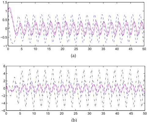
−0.0134±0.2474i, and γ = 0.0134. It is easy to check that the conditions of Lemma 2.4 and Lemma 2.5 hold. When time delays are selected as τ1 = 0.012,τ2 = 0.015,τ3 = 0.02, and τ1 = 0.12,τ2 = 0.15,τ3 = 0.2, respectively, we see that τ¯(kA1k+kγB1k)kB1k < 0.2·(1.0350.0134+0.029)·0.029 = 0.4605 < 1. From Theorem 3.1, system (2.1) generates a partial periodic oscillation (see Fig- ures4.1a and4.1b). When delays are increased, the convergent rate is slightly changed (see Figures4.2aand4.2b).
When we select ε1 = 0.35,ε2 = 0.25,ε3 = 0.15;Ω21 = 0.96,Ω22 = 1.25,Ω23 = 2.15;κ1 = 0.2,κ2 =0.5,p1 =1.15,p2 =1.25,p3=1.85,q1=0.75,q2=0.65,q3=0.85, and delays are τ1= 0.2,τ2 = 0.4,τ3 =0.5, and τ1 =1,τ2 =2,τ3= 2.5, respectively, then the eigenvalues of matrix Aare 0.1750±0.9460i,−0.1250±1.0651i,−1.3932, and 1.5432. Note that 1.5432 > 0, and the conditions of Theorem3.4are satisfied. Thus, system (2.1) generates a periodic oscillation (see Figures4.3 and4.4).
50 100 150 200 250 300
4
2 0 2 4
(a)
0 50 100 150 200 250 300
4
2 0 2 4
(b)
Figure 4.1: (a) u1(t),u2(t), andu3(t)are convergent; delays: 0.012, 0.015, 0.020.
Solid line: u1(t), dashed line: u2(t), dashdotted line: u3(t). (b) u4(t)is conver- gent, both u5(t)andu6(t)are oscillatory; delays: 0.012, 0.015, 0.020. Solid line:
u4(t), dashed line: u5(t), dashdotted line:u6(t).
0 50 100 150 200 250 300
4
2 0 2 4
(a)
0 50 100 150 200 250 300
−10
−5 0 5 10
(b)
Figure 4.2: (a) u1(t),u2(t), and u3(t) are convergent; delays: 1.2, 1.5, 2. Solid line: u1(t), dashed line: u2(t), dashdotted line: u3(t). (b) u4(t)is convergent, bothu5(t)andu6(t)are oscillatory; delays: 1.2, 1.5, 2. Solid line: u4(t), dashed line: u5(t), dashdotted line: u6(t).
0 5 10 15 20 25 30 35 40 45 50
1
0.5 0 0.5 1 1.5
(a)
0 5 10 15 20 25 30 35 40 45 50
6
4
2 0 2 4 6
(b)
Figure 4.3: Oscillation of the solution; delays: 0.02, 0.04, 0.05. (a) Solid line:
u1(t), dashed line: u2(t), dashdotted line: u3(t). (b) u4(t), dashed line: u5(t), dashdotted line: u6(t).
0 5 10 15 20 25 30 35 40 45 50
1.5
1
0.5 0 0.5 1 1.5
(a)
0 5 10 15 20 25 30 35 40 45 50
−10
−5 0 5 10
(b)
Figure 4.4: Oscillation of the solution; delays: 0.2, 0.4, 0.5. (a) Solid line: u1(t), dashed line: u2(t), dashdotted line: u3(t). (b) u4(t), dashed line: u5(t), dashdot- ted line: u6(t).
5 Conclusion
This paper discussed a system of two coupled damped Duffing oscillators driven by a van der Pol oscillator with delays. Some sufficient conditions to ensure the periodic and partial peri- odic oscillations for the system are established. Interestingly, this partial periodic oscillation is induced by unbalanced damped oscillators. When periodic and partial periodic oscillations occur, delays only affect the oscillation frequency. The study of micro-electro-mechanical phe- nomena and nano-electro-mechanical phenomena often requires experimental methods that can accurately control and manipulate the interaction between micro- and nano-objects. Our results are helpful for developing of novel MEMS or NEMS devices, which can precisely con- trol of these nanoscale interactions, provide an ideal platform for interacting with the micro- and nano-world.
Acknowledgements
This work was supported by the SECURE Cybersecurity Center of Excellence and the Center of Excellence for Communication Systems Technology Research (CECSTR) at Prairie View A&M University.
References
[1] N. Chafee, A bifurcation problem for a functional differential equation of finitely retarded type, J. Math. Anal. Appl. 35(1971), 312–348. https://doi.org/10.1016/
0022-247X(71)90221-6
[2] C. H. Feng, R. Plamondon, An oscillatory criterion for a time delayed neural ring net- work model, Neural Networks 29–30(2012), 70–79. https://doi.org/10.1016/j.neunet.
2012.01.008
[3] P. Ghorbaniana, S. Ramakrishnana, A. Whitmanb, H. Ashrafiuona, A phenomeno- logical model of EEG based on the dynamics of a stochastic Duffing–van der Pol oscillator network, Biomed. Sign. Proc. Control. 15(2015), 1–10.https://doi.org/10.1016/j.bspc.
2014.08.013
[4] Z. Ghouli, M. Hamdi, F. Lakrad, M. Belhaq, Quasiperiodic energy harvesting in a forced and delayed Duffing harvester device,J. Sound Vibrat. 407(2017), 271–285. https:
//doi.org/10.1016/j.jsv.2017.07.005
[5] J. Guckenheimer, P. Holmes, Nonlinear oscillations, dynamical systems and bifurcations of vector fields, Applied Mathematical Sciences, Vol. 43, Springer-Verlag, 1983.https://doi.
org/10.1007/978-1-4612-1140-2
[6] H. Y. Hu, Global Dynamics of a Duffing system with delayed velocity feedback, in: Rega G., Vestroni F. (eds),IUTAM Symposium on Chaotic Dynamics and Control of Systems and Pro- cesses in Mechanics, Solid Mechanics and its Applications, Vol. 122, Springer, Dordrecht, 2005, pp. 335–344.https://doi.org/10.1007/1-4020-3268-4_32