5J=>EEJO B A?D=E?= 5OIJAI MEJD 8=HOEC 6EA ,A=OI

(1)

Stability of Mechanical Systems with Varying Time Delays

Tamás Insperger

Dissertation for the Title Doctor of the Hungarian Academy of Sciences

May, 2014

(2)

Chapter 1 Introduction

Dynamical systems described with dierential equations often come up in dierent eld of science and engineering. A dierential equation can serve as a model for how the rate of change of state depends on the present state of a system. However, the rate of change of state may depend on past states, too. It has been known for a long time that several problems can be described by models including past eects. One of the classical examples is the predatorprey model of Volterra [230], where the growth rate of predators depends not only on the present quality of food (say, prey), but also on past quantities (in the period of gestation, say). The rst delay models in engineering appeared for wheel shimmy [190] and for ship stabilization [157] in the early 1940s.

There are several other engineering applications in which time delay plays a crucial role. As recognized in the late 1940s with the development of control theory, time delay typically arises in feedback control systems due to the nite speed of information transmission and data processing [228, 204]. Another typical application is the stability of machining processes, where time delay appears due to the surface regeneration by the cutting edge [223, 226, 209, 5]. Similar equations describe the car-following trac models involving the reaction time of drivers [173], or the active suspension of cars with a time delay in driver's response [176, 177, 68]. Time delay also plays important role in neural networks [35, 174], in human motion control [213, 155, 10] and in epidemiology models [186, 2].

Systems whose rate of change of state depends on states at deviating arguments are generally described by functional dierential equations (FDEs). According to Myshkis [164], FDEs are equations involving the function x(t) of one scalar argument t (called time) and its derivatives for several values of argument t. The literature on FDEs is quite extensive. Several books have appeared summarizing the most important theorems; see, for instance, the books by Myshkis [164], Bellman and Cooke [19], Èl'sgol'c [54], Halanay [77], Hale [78], Driver [51], Kolmanovskii and Nosov [127], Hale and Lunel [79], Diekmann et al. [44], just to mention a few. There are also several

1

(5)

books dealing with dierent applications and numerical techniques; see for instance, Stépán [206], Niculescu [168], Bellen and Zennaro [18], Gu et al. [71], Zhong [243], Michiels and Niculescu [152], Erneux [58], Balachandran et al. [15], Yi et al. [239], and Insperger and Stépán [115].

RFDE is a mathematical terminology. In the engineering literature, RFDEs are referred to as delay-dierential equations (DDEs), or simply delay equations. In this dissertation, we follow the latter terminology, and use the term DDE rather than RFDE.

In this dissertation, dierent engineering problems are considered that are all described with DDEs with varying time delays. Chapter 2 gives a brief overview on some special cases of linear DDEs with time-periodic coecients. Then each chapter is related to a thesis of the dissertation.

Chapter 3 presents an ecient numerical method, the so-called rst-order semi- discretization, for the stability analysis of linear time-periodic DDEs. A basic version of the semi-discretization method (called zeroth-order semi-discretization) was presented by Insperger and Stépán [100, 104]. The point of the method is that the time-delayed terms are discretized, the time-periodic coecients are approximated by piecewise constant ones, while the actual time-domain terms are left in their original form during the discretization process. The new result given in Thesis 1 is related to the convergence of the discretization method with respect to the order of the approximation of the delayed term. It is shown that if the periodic coecients are approximated by piecewise constant ones then the zeroth-order approximation gives a discretization error proportional to the square of the discretization step, while the rst- and any higher-order approximation gives a discretization error proportional to the cube of the discretization step. This result was published in Insperger et al. [110] and was also included into the book Insperger and Stépán [115].

In Chapter 4, a two-degrees-of-freedom model of turning processes is presented, where state-dependent regenerative delays arise in the model equations. DDEs with state-dependent delays are strongly nonlinear, since the state appears in its own argument through the time delay, i.e., the nonlinearity in the systems is dened by the solution. The new result given in Thesis 2 is the application of the linearization technique of Hartung and Turi [82] to the model equations. It is shown that the linear stability boundaries are slightly dierent from that of the constant delay model due to the dependence of the instantaneous chip thickness on the regenerative delay. This result was published by Insperger et al. [108].

Chapter 5 presents a single-degree-of-freedom model of milling processes with varying spindle speed. The corresponding mechanical model is a DDE with time-periodic delay. As a new result, the stability charts are determined for the model in the plane

(6)

of the spindle speed and the axial depth of cut using the rst-order semi-discretization method. It is shown that multiple lobes appears at the location of the ip lobes of the constant-spindle-speed milling. These results are composed in Thesis 3, and were also published in the book Insperger and Stépán [115]. Experimental verication of suppressing period doubling chatter by spindle speed variation is also presented according to the joint papers Seguy et al. [193, 194] that were made in collaboration with French partners. The experiments were performed by Sebastien Seguy (École Nationale d'Ingénieurs de Tarbes, France), who made his PhD on this topic in 2008 [192]. The experimental results are not included into Thesis 3, but they are presented for the sake of completeness.

Chapter 6 presents the so called act-and-wait control technique for systems with feedback delays. The act-and-wait controller is a special case of periodic controllers where the feedback is periodically switched o and on. Control systems with feedback delays are described by DDEs associated with innite-dimensional state spaces. Conse- quently, the stability of the control process is determined by innitely many eigenvalues (poles) that all should be monitored during the adjustment of the control parameters.

It is shown that if the act-and-wait control technique is applied such that the waiting (switch-o) period is larger than the feedback delay, then the system can be described by a nite-dimensional discrete map, and only nite number of eigenvalues should be considered during the stabilization process. This result is composed in Thesis 4 and was published in Insperger [106] and also in the book Insperger and Stépán [115].

Chapter 7 deals with a force control process in the presence of feedback delay.

Here, the goal is to reduce the error of the contact force between the actuator and the environment. In order to achieve this goal, the proportional gain in the controller should be increased, but on the other hand, for large proportional gains, the system looses stability due to the feedback delay. It is shown that the proportional gain and, consequently, the accuracy of the contact force can be increased by the application of the act-and-wait control concept without loosing stability. The results are composed in Thesis 5 and were published in Insperger et al. [111] and also in the book Insperger and Stépán [115].

(7)

Chapter 2 Mathematical background

Since most of the theses in this dissertation are related to time-periodic DDEs, an overview is given in this chapter on the related mathematical theory. In the next sections, some basic properties of some special classes of dierential equations, namely, linear autonomous ordinary dierential equations (ODEs), linear time-periodic ODEs, linear autonomous DDEs, linear time-periodic DDEs and DDEs with state-dependent delays are summarized briey.

2.1 Linear Autonomous ODEs

Linear autonomous ordinary dierential equations (ODEs) have the general form

˙

x(t) =Ax(t), (2.1)

wherex(t)∈Rⁿ, A is an n×n matrix, and

˙ x= dx

dt = col (dx1

dt dx2

dt · · · dxn

dt )

with x₁, x₂, . . . , x_n being the elements of vector x. For a given initial value x(0), the solution of (2.1) can be written in the form

x(t) = e^Atx(0) , (2.2) where e^At is the exponential of matrix At, dened by the Taylor series of the exponential function (see Appendix A). For a general overview on matrix exponentials, see the book of Hirsch and Smale [90], or the book of Perko [179].

The stability of the trivial solution x(t) ≡ 0 is determined by the eigenvalues λ_j, j = 1,2, . . . , n, of the coecient matrix A. These eigenvalues are the characteristic exponents of (2.1), but they are often called characteristic roots or poles, too. If each

4

(8)

λ_j is unique in the minimal polynomial of A, then each solution of (2.1) can be written in the form

x(t) =

∑n j=1

C_je^λ^j^t, (2.3)

with C_j ∈ Cⁿ being appropriate vectors depending on the initial condition. If the characteristic exponents have negative real parts, i.e.,Reλ_j <0 for all j = 1,2, . . . , n, then the trivial solution of (2.1) is asymptotically stable. In the general case, the characteristic exponents can be determined by solving the characteristic equation

det (λI−A) = 0, (2.4)

where I stands for the n × n identity matrix. Development of (2.4) results in an nth-degree polynomial of λ, whose roots (i.e., the characteristic exponents) can be determined by a number of numerical methods. Stability analysis, however, does not require the exact calculation of the characteristic exponents; only the sign of the real part of the critical (i.e., rightmost) exponent must be determined. This analysis can be performed by the celebrated RouthHurwitz criterion [187, 95], which gives a necessary and sucient condition for stability based on the coecients of the characteristic polynomial.

Depending on the location of the critical characteristic exponents, there are two typical mechanisms for loss of stability of linear autonomous systems [72]:

1. The critical characteristic exponents form a complex conjugate pair moving from the left-hand side of the complex plane to the right-hand side; they cross the imaginary axis, as shown by case (a) in Figure 2.1. This case is an essential necessary condition for the so-called Hopf (or AndronovHopf or PoincaréAndronov Hopf ) bifurcation of the corresponding nonlinear system, for which the equation under analysis is the variational system. The systematic study of the conditions and a proof of the corresponding bifurcation theorem have been done by An- dronov and Leontovich [8] for the two-dimensional case, and by Hopf [92] for the n-dimensional case. According to the theory of nonlinear systems, either stable or unstable periodic motion may exist around the equilibrium of the corresponding nonlinear system, called supercritical and subcritical bifurcation, respectively.

2. The critical characteristic exponent is a real one moving from the left-hand side of the complex plane to the right-hand side through the origin, as shown by case (b) in Figure 2.1. This case is called saddle-node bifurcation of the corresponding nonlinear system.

(9)

Figure 2.1: Critical characteristic exponents for linear autonomous ODEs: (a) Hopf bifurcation, (b) and saddle-node bifurcation.

2.2 Linear Periodic ODEs

The general form of linear periodic ODEs reads

˙

x(t) = A(t)x(t), A(t) =A(t+T), (2.5) with x(t) ∈ Rⁿ. Here, the n ×n coecient matrix A(t) is time-periodic at period T, called the principal period in contrast to the constant-coecient matrix of the autonomous system (2.1). The main theorems on general periodic systems are summarized in the book of Farkas [60].

For periodic ODEs, a stability condition is provided by the Floquet theory [61]. The solution of (2.5) with the initial conditionx(0)is given byx(t) = Φ(t)x(0), whereΦ(t) is a fundamental matrix of (2.5). According to the Floquet theory, the fundamental matrix can be written in the form Φ(t) = P(t) e^Bt, where P(t) = P(t +T) is a periodic matrix with initial value P(0) = I, and B is a constant matrix. The matrix Φ(T) = e^BT is called the monodromy matrix (or principal matrix or Floquet transition matrix) of (2.5). This matrix gives the connection between the initial state and the state one principal period later: x(T) =Φ(T)x(0).

The eigenvalues ofΦ(T)are the characteristic multipliers (µ_j,j = 1,2, . . . , n) (also called Floquet multipliers or the poles ofΦ(T)) calculated from

det(µI−Φ(T)) = 0. (2.6)

The eigenvalues of matrixB are the characteristic exponents (λ_j,j = 1,2, . . . , n) given by

det(λI−B) = 0. (2.7)

If µ is a characteristic multiplier, then there are characteristic exponents λ such that µ = exp(λT), and vice versa. Due to the periodicity of the complex exponential function, each characteristic multiplier is associated with innitely many characteristic exponents of the formλk =γ+i (ω+k2π/T), whereγ, ω ∈R,k ∈Z, andT ω∈(−π, π].

(10)

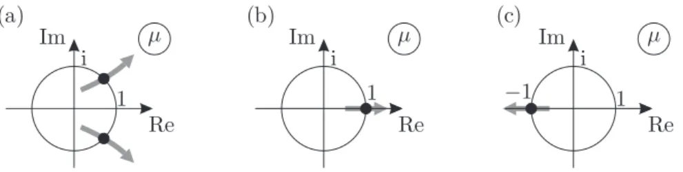
Figure 2.2: Critical characteristic multipliers for periodic systems: (a) secondary Hopf bifurcation, (b) cyclic-fold bifurcation, and (c) period-doubling bifurcation.

The trivial solution x(t) ≡0 of (2.5) is asymptotically stable if and only if all the characteristic multipliers have modulus less than one, that is, all the characteristic exponents have negative real parts.

Similarly to autonomous systems, the basic types of loss of stability can be classied according to the location of the critical characteristic multipliers [72]. For periodic systems, there are three typical cases:

1. The critical characteristic multipliers form a complex conjugate pair crossing the unit circle, i.e., |µ|= 1 and|µ¯|= 1, as shown by case (a) in Figure 2.2. This case is topologically equivalent to the Hopf bifurcation of autonomous systems and is called secondary Hopf (or NeimarkSacker) bifurcation.

2. The critical characteristic multiplier is real and crosses the unit circle at +1, as shown by case (b) in Figure 2.2. The bifurcation that arises is topologically equivalent to the saddle-node bifurcation of autonomous systems and is called cyclic-fold (or period-one) bifurcation.

3. The critical characteristic multiplier is real and crosses the unit circle at −1, as shown by case (c) in Figure 2.2. There is no topologically equivalent type of bifurcation for autonomous systems. This case is called period-doubling (or period-two or ip) bifurcation.

Generally, the monodromy matrix cannot be determined in closed form, but there exist several numerical and semi-analytical techniques to approximate it, such as Hill's innite determinant method and its generalizations [89, 215, 22, 166], the method of strained parameters [166], the method of multiple scales [166], and the Chebyshev polynomial approach [201, 202]. A simple numerical method is the piecewise constant approximation of the periodic matrixA(t)in the form

A(t)≈A_i :=

∫ ih (i−1)h

A(s) ds , t∈[t_i, t_i+1), (2.8)

(11)

wheret_i =ihis the discrete time withi∈Z,h=T /pis the length of the discretization step, and pis an integer [94, 60]. The original system can be approximated by

y(t) =˙ A_iy(t), t∈[t_i, t_i+1), (2.9) for which the solution over a discretization interval is

y(t_i+1) = e^Aⁱ^hy(t_i). (2.10) Application of (2.10) overprepeated discretization steps with initial state y(0) results in

y(T) = ˜Φ(T)y(0) , (2.11)

where

Φ(T˜ ) = eÂ^p⁻¹^h eÂ^p⁻²^h · · · eÂ⁰^h (2.12) is an approximation for the monodromy matrix Φ(T). Eigenvalue analysis of Φ(T˜ ) gives then an approximate description of the stability properties of (2.5). A higher- order generalization of this piecewise constant approximation technique is the method of Magnus expansion, which involves higher-order terms of the so-called Magnus series of the logarithm of the fundamental matrix Φ(h) (see, e.g., [145, 116, 117, 32]).

Approximation (2.8) corresponds to the rst-order Magnus expansion ofln( Φ(h))

.

2.3 Linear Autonomous DDEs

The general form of linear autonomous DDEs is

˙

x(t) =L(x_t), (2.13) whereL:C →Rⁿis a continuous linear functional (Cis the Banach space of continuous functions) and the continuous functionx_t is dened by the shift

x_t(ϑ) =x(t+ϑ), ϑ ∈[−σ,0]. (2.14) According to the Riesz representation theorem (see [78]), the linear functional L can be represented in the matrix form

L(x_t) =

∫ 0

−σ

dη(ϑ)x(t+ϑ), (2.15)

where η : [−σ,0]→ Rⁿ^×ⁿ is a matrix function of bounded variation, and the integral is a Stieltjes one, i.e., (2.15) contains both point delays and distributed delays.

(12)

The characteristic equation can be obtained by substituting the nontrivial solution x(t) = C e^λt, C∈Cⁿ, into (2.13), which gives

det (

λI−

∫ ₀

−σ

e^λϑdη(ϑ) )

| {z }

:=D(λ)

= 0 . (2.16)

The left-hand side of this equation denes the characteristic function D(λ) of (2.13).

The characteristic exponents are the zeros of the characteristic function. As opposed to the characteristic polynomial of autonomous ODEs, the characteristic functionD(λ) has, in general, an innite number of zeros in the complex plane, all of which should be considered during the stability analysis. Stability charts that present the stability properties as a function of the system parameters have therefore a rich and intricate structure even for the simplest DDEs.

Linear autonomous DDEs containing only point/discrete delays can be given in the form

˙

x(t) = Ax(t) +

∑g j=1

B_jx(t−τ_j), (2.17)

where A and the B_j's are n×n matrices, τ_j > 0 for all j, and g ∈ Z⁺. In this case, only discrete values of the past have inuence on the present rate of change of state.

An example of a DDE with distributed delay is

˙

x(t) = Ax(t) +

∫ ₋_σ₂

−σ1

K(ϑ)x(t+ϑ) dϑ , (2.18)

where K(ϑ) is an n× n measurable kernel function, σ₁, σ₂ ∈ R, and σ₁ > σ₂ ≥ 0. The kernel function K(ϑ) describes the weight of the past eects over the interval [t−σ₁, t−σ₂]. If the kernel is a constant matrix multiplied by the shifted Dirac delta distribution, i.e., K(ϑ) = K0δ(ϑ+τ) with σ1 ≤ τ ≤ σ2, then the integral in (2.18) gives the point delayK₀x(t−τ).

Linear autonomous DDEs with distributed delay and with a nite number of point delays can be given in the general form

˙ x(t) =

∫ ₀

−σ

K(ϑ)x(t+ϑ) dϑ , (2.19) where K(ϑ) is an n×n measurable kernel function that may comprise a measurable distribution and nitely many shifted Dirac delta distributions. That is,K(ϑ)can also be given in the form

K(ϑ) =W(ϑ) +

∑g j=1

Bjδ(ϑ+τj), (2.20)

(13)

where W(ϑ) is an n×n measurable function (a weight function), the B_j's are n×n constant matrices,δ(ϑ)denotes the Dirac delta distribution,τ_j ≥0for allj, andg ∈N.

Thus, (2.19) can be written as

˙ x(t) =

∫ 0

−σ

W(ϑ)x(t+ϑ)dϑ+

∑g j=1

B_jx(t−τ_j). (2.21) A necessary and sucient condition for the asymptotic stability of DDE (2.13) with (2.15) is that all the innite number of characteristic exponents have negative real parts and there exist a scalar ν >0 such that

∫ 0

−∞

e⁻^νϑ|dηjk(ϑ)|<∞, j, k = 1,2, . . . , n , (2.22) where η_jk(ϑ) are the elements of η(ϑ). Condition (2.22) means that the past eect decays exponentially in the past. Obviously, this condition holds ifσ in the lower limit of the integral in (2.15) is nite.

Although there are innitely many characteristic exponents, it is not necessary to compute all of them, since stability analysis requires only the sign of the real part of the rightmost one(s). There exist several analytical and semi-analytical methods to derive the stability conditions for the system parameters. The rst attempts for determining stability criteria for rst- and second-order scalar DDEs were made by Bellmann and Cooke [19] and by Bhatt and Hsu [20]. They used the D-subdivision method of Neimark [167] combined with a theorem of Pontryagin [181]. The book of Kolmanovskii and Nosov [127] summarizes the main theorems on the stability of DDEs, and contains several examples as well. A sophisticated method was developed by Stépán [206] (generalized also by Hassard [86]) that can be applied even for a combi- nation of multiple point delays and for distributed delays. There exist several ecient numerical methods to determine the rightmost exponents for a delayed system; see, for instance, the celebrated DDE-BIFTOOL developed by Engelborghs et al. [56, 57], the pseudospectral dierencing method by Breda et al. [23, 24], the cluster treatment method by Olgac and Sipahi [171, 172], the Galerkin projection by Wahi and Chat- terjee [231, 232], the mapping algorithm by Vyhlídal and Zítek [229], the harmonic balance by Liu and Kalmár-Nagy [143], or the Lambert W function approach by Ulsoy et al. [11, 238].

The stability properties of DDEs are often represented in the form of stability charts that show the stable and unstable domains, or alternatively, the number of unstable characteristic exponents (also called instability degree) in the space of system parameters. Stability charts for autonomous DDEs can be constructed by the D- subdivision method. The curves where changes in the number of unstable exponents

(14)

happen are given by the so-called D-curves (also called exponent-crossing curves or transition curves) given by

R(ω) = 0, S(ω) = 0, ω∈[0,∞), (2.23) where

R(ω) := ReD(iω), S(ω) := ImD(iω), (2.24) with D(λ) being the characteristic function dened in (2.16) and ω the parameter of the curves [209]. Due to the continuity of the characteristic exponents with respect to changes in the system parameters (see, for instance, [152]), the D-curves separate the parameter space into domains where the numbers of unstable characteristic exponents are constant. The determination of these numbers for the individual domains is not a trivial task. One technique is to calculate the exponent-crossing direction (also called root-crossing direction or root tendency) along the D-curves, which is the sign of the partial derivative of the real part of the characteristic exponent with respect to one of the system parameters. If the number of unstable exponents is known for at least one point in one domain, then it can be determined for all the other domains by considering the exponent-crossing direction along the D-curves. The stability boundaries are the D-curves bounded the domains with zero unstable characteristic exponent.

Alternatively, Stépán's formulas [206] can also be used to determine the number of unstable characteristic exponents in a simple and elegant way. This technique requires the analysis of the functionsR(ω) and S(ω) dened in (2.24) only, without the analysis of the exponent-crossing direction. Assume that the characteristic function D(λ)associated with (2.13) has no zeros on the imaginary axis and (2.22) holds. If the dimension n of (2.13) is even, i.e., n = 2m with m being an integer, then the number of unstable exponents is

N =m+ (−1)^m

∑r k=1

(−1)^k+1sgnS(ρ_k), (2.25) where ρ₁ ≥ · · · ≥ ρ_r > 0 are the positive real zeros of R(ω). If the dimension n of (2.13) is odd, i.e., n = 2m+ 1 with m being an integer, then the number of unstable exponents is

N =m+1

2 + (−1)^m (

1

2(−1)^ssgnR(0) +

s−1

∑

k=1

(−1)^ksgnR(σ_k) )

, (2.26)

where σ₁ ≥ · · · ≥ σ_s = 0 are the nonnegative real zeros of S(ω). For further details and for an exact proof, see Theorems 2.15 and 2.16 in [206].

(15)

2.4 Linear Time-Periodic DDEs

Linear time-periodic DDEs have the general form

˙

x(t) =L(t,x_t), L(t+T) =L(t), (2.27) wherex_t is a continuous function dened by (2.14),L:R×C →Rⁿ is continuous and linear in x_t. According to the Riesz representation theorem, the functional L can be written in the Stieltjes integral form

L(t,x_t) =

∫ ₀

−σ

d_ϑη(t, ϑ)x(t+ϑ), (2.28) whereη:R×[−σ,0]→R^n×n is a matrix function of bounded variation inϑ ∈[−σ,0].

Linear time-periodic DDEs with constant point delays can be dened as

˙

x(t) = A(t)x(t) +

∑g j=1

B_j(t)x(t−τ_j), (2.29) A(t+T) =A(t), B_j(t+T) = B_j(t),

where A(t) and the B_j(t)'s are n×n matrices, τ_j > 0 for all j, and g ∈ Z⁺. Linear time-periodic DDEs with distributed delay read

˙

x(t) = A(t)x(t) +

∫ ₋σ2

−σ1

K(ϑ, t)x(t+ϑ) dϑ , (2.30) A(t+T) =A(t), K(ϑ, t+T) = K(ϑ, t),

whereK(ϑ, t)is the time-periodicn×nkernel function,σ₁, σ₂ ∈R, andσ₁ > σ₂ ≥0. A special case of (2.30) occurs when the kernel function is a constant matrix multiplied by a time-periodic Dirac delta distribution, i.e.,K(ϑ, t) =K₀δ(ϑ−τ(t))withσ₁ ≤τ(t)≤ σ₂ andτ(t+T) = τ(t). In this case, the integral in (2.30) gives the time-periodic point delayK₀x(t−τ(t)). The general form of linear time-periodic DDEs with time-periodic point delays is

x(t) =˙ A(t)x(t) +

∑g j=1

B_j(t)x(t−τ_j(t)), (2.31) A(t+T) = A(t), B_j(t+T) =B_j(t), τ_j(t+T) = τ_j(t).

Linear time-periodic DDEs with distributed delay and with a nite number of point delays can be given in the general form

˙ x(t) =

∫ ₀

−σ

K(ϑ, t)x(t+ϑ) dϑ , (2.32)

(16)

whereK(ϑ, t) is an n×n measurable kernel function that can be written in the form K(ϑ, t) =W(ϑ, t) +

∑g j=1

Bj(t)δ(ϑ+τj(t)). (2.33) Here W(ϑ, t+T) = W(ϑ, t) is a time-periodic n ×n measurable function (a time- periodic weight function), Bj(t +T) = Bj(t) are n×n time-periodic matrices, δ(ϑ) denotes the Dirac delta distribution, τ_j(t) ≥0 for all j, and g ∈ N. Thus, (2.32) can be written as

˙ x(t) =

∫ ₀

−σ

W(ϑ, t)x(t+ϑ)dϑ+

∑g j=1

B_j(t)x(t−τ_j(t)). (2.34) According to the Floquet theory of DDEs [76, 79], the solution segmentxtfor (2.27) associated with the initial function x₀ can be given as x_t =U(t)x₀, where U(t) is the solution operator (innitesimal generator). The stability of the system is determined by the spectrum of the corresponding monodromy operatorU(T). The nonzero elements of the spectrum ofU(T)are called characteristic multipliers (also referred to as Floquet multipliers or poles) and are dened by

Ker(µI − U(T))\ {0} ̸=∅, µ̸= 0, (2.35) or

Ker(µI − U(T))̸={0}, µ̸= 0, (2.36) with I denoting the identity operator. Generally, time-periodic DDEs have innitely many characteristic multipliers. If µis a characteristic multiplier, and µ = e^λT, then λ is called the characteristic exponent. Similarly to linear periodic ODEs, each characteristic multiplier is associated with innitely many characteristic exponents of the formλ_k =γ+ i (ω+k2π/T), whereγ, ω ∈R, k ∈Z, and T ω∈(−π, π].

A necessary and sucient condition for the asymptotic stability of the time-periodic DDE (2.27) with (2.28) is that all the characteristic multipliers have modulus less than one (that is, all the characteristic exponents have negative real parts) and there exist a scalarν >0 such that

∫ ₀

−∞

e⁻^νϑ|d_ϑη_jk(t, ϑ)|<∞, j, k= 1,2, . . . , n , (2.37) for all t ∈ R, where η_jk(t, ϑ) are the elements of η(t, ϑ). Similarly to autonomous DDEs, condition (2.37) trivially holds ifσ in the lower limit of the integral in (2.28) is nite. The diculty in the stability analysis of periodic DDEs is that the monodromy operator U(T) has generally no closed form; consequently, the stability conditions cannot be derived in an analytic form.

(17)

There exist several numerical and semi-analytical techniques to determine the stability conditions for periodic DDEs. Most of them were developed with the aim of constructing stability charts for milling processes. Insperger and Stépán [100] introduced the semi-discretization method that is based on a special discretization of the individual terms in the DDE. Budak and Altintas [26, 27] and Merdol and Altintas [150] developed the multi-frequency solution method, which is a kind of alternative application of Hill's innite determinant method. Butcher et al. [30, 33] used an expansion of the solution in terms of Chebyshev polynomials to obtain an approximate monodromy matrix. A temporal nite element method using Hermite polynomials was developed by Bayly et al. [17] for interrupted turning, and formulated to general periodic DDEs by Mann and Patel [147]. Szalai et al. [219] used the characteristic matrices of the system to derive stability charts (see also [200]). Recently, Khasawneh and Mann presented an eective numerical algorithm called the spectral element method that is a temporal nite element method involving highly accurate numerical quadratures for the integral terms [121, 122].

2.5 DDEs with state-dependent delays

If the delay depends not only on the time but also on the state, then the corresponding equation is called a DDE with state-dependent delay (SD-DDE). A simple example for SD-DDEs is

˙

x(t) =Ax(t) +B x(t−τ(t,x(t))) (2.38) with τ(t,x(t)) ≥ 0. Here, the delay depends on the actual time t and on the actual state x(t). If the delay depends also on delayed values of the state, then it is usually written in the formτ(t,xt)≥0, where xt is dened as in equation (2.14).

State-dependent delays arose rst in the two-body problem of classical electrody- namics [50], but they appear in many other elds, such as population models [169, 135], automatic position control [233], neural networks models [16], and machine tool vibration theory [108]. There are several papers dealing with some special classes of systems with state-dependent delays [80, 133, 134]. A survey about DDEs with state-dependent delays is given in [85].

SD-DDEs are always nonlinear, since the state appears in its own argument. Thus, the nonlinearity is dened by the solution of the system. The corresponding linear system is, however, a DDE with constant (or time-dependent) delay. Linearization of SD-DDEs is complicated by the fact that the solution of the system is not dierentiable with respect to the state-dependent delay (see, e.g., [81] and the references therein).

Consequently, true linearization is not possible, rather we are looking for a linear

(18)

DDE, which is associated to the original system in the sense that they have the same local stability properties. For example, consider the autonomous scalar SD-DDE

˙

x(t) =x(t−(τ₀+x(t))) . (2.39)

This is a nonlinear equation due to the state-dependent time delayτ(x(t)) = τ0+x(t). The DDE

˙

y(t) = y(t−τ₀) (2.40)

with constant time delay is a linear system that can be considered as a linear variational system corresponding to (2.39) around the equilibrium x= 0. In our terminology, linearization means that the trivial solutions y(t) ≡ 0 of (2.40) and x(t) ≡ 0 of (2.39) are asymptotically stable at the same time. Linearization techniques for general autonomous SD-DDEs were given by Hartung and Turi [82] and for time-periodic SD-DDEs by Hartung [83]. The mathematical background for the full-discretization of DDEs with state-dependent delays was presented by Gy®ri et al. [73, 74].

In engineering practice, DDEs with state-dependent delay are rarely used since the appropriate mathematical tools, like linearization techniques, have just been developed recently (see [82, 83]), and these new results have not been adopted in engineering problems yet. Still, the eect of state-dependent delay becomes important in rotary cutting processes (e.g., in milling, or drilling) where the torsional vibrations of the tool are signicant in the system's dynamics. Richard et al. [184] and Germay et al.

[67] investigated drilling with drag bits and showed that state-dependent regenerative delay arises due to the torsional vibration of the tool. They investigated self-excited vibrations and periodic orbits of the tool numerically. Insperger et al. [105] showed that state-dependent delay arises in the governing equation of the milling process even when only the bending oscillation of the tool is considered and its torsional compliance is neglected. The stability analysis for the same system was performed by Bachrathy et al. [14]. The state-dependency of the regenerative delay due to the bending compliance of the milling tool was also derived by Long et al. [144].

(19)

Chapter 3 Higher-order semi-discretization method

The semi-discretization method was introduced by Insperger and Stepan [100] for general time-periodic DDEs. This method was later referred to as zeroth-order semi- discretization. Elbeyli and Sun [53] generalized the method to the so-called improved zeroth-order (see also [104]) and the rst-order semi-discretization for second-order scalar systems. The general higher-order formalism was presented in [110]. The convergence of the method was established by Hartung et al. [84] for a large class of DDEs appearing in engineering applications. It was shown that semi-discretization preserves asymptotic stability of the original equation; therefore it can be used to construct approximate stability charts.

The merit of the semi-discretization method is that it can be used eectively to determine stability charts for time-periodic DDEs arising in dierent engineering problems while the numerical scheme itself is relatively simple. One of the main elds of application of semi-discretization is the stability prediction for machining processes.

Dierent milling models were analyzed by Gradi²ek et al. [70], Henninger and Eber- hard [87, 88], Sims et al. [203], Dombovari et al. [48], Bachrathy et al. [13], and Wan et al. [234] using the semi-discretization method. Ding et al. [45, 46] applied an alternative semi-discretization method for the milling problem using a slightly dierent concept in the discretization scheme (see also [112]). Sellmeier and Denkena [195] applied the method to milling processes with uneven tooth pitches and pointed out that the method can be considered an extension of the theory of sampled control systems with feedback delay according to Ackermann [1] (see also [137, 12, 170]).

A continuous-time approximation technique was introduced by Sun and Song [216, 217] based on the concept of semi-discretization that can handle multiple time delays for both linear and nonlinear dynamical systems. Models with time-periodic delays

16

(20)

were considered by Insperger and Stépán [103], Long et al. [144], Faassen et al. [59], Zatarain et al. [241], and Seguy et al. [193]. The method can also be used for other models, for instance, for the stability analysis of periodic control systems with delayed feedback, as was shown by Sheng et al. [197] and by Konishi and Hara [128].

In this chapter, rst, the general formulas for the higher-order semi-discretization method are presented. Then the zeroth- and the rst-order techniques are described in detail. After that, rate of convergence estimates are given. The new results are composed in Thesis 1 at the end of the chapter. The results presented here were published in Insperger et al. [110] and was also included into the book Insperger and Stépán [115].

3.1 General formulas

Consider the time-periodic DDE with multiple time-periodic point delays of the form x(t) =˙ A(t)x(t) +

∑g j=1

B_j(t)u(t−τ_j(t)), (3.1)

u(t) =Dx(t), (3.2)

wherex(t)∈Rⁿ is the state,u(t)∈R^m is the input,A(t+T) = A(t)and B_j(t+T) = B_j(t), j = 1,2, . . . , g, are n×n and n×m time-periodic matrices, respectively, D is an m×n constant matrix, and τ_j(t+T) = τ_j(t) > 0, j = 1,2, . . . , g. The principal period of the system isT. Note that (3.1)(3.2) can also be written in the form

˙

x(t) = A(t)x(t) +

∑g j=1

B_j(t)Dx(t−τ_j(t)). (3.3) The main point of higher-order semi-discretization methods is that the time-periodic coecients and the time-periodic delays are approximated by piecewise constant functions, the delayed terms are approximated by linear combinations of some discrete delayed values of the state variable x, while the nondelayed terms are left in their original form. Consider the discrete time scale t_i = ih, i ∈ Z, such that the time step ish=T /pwith pbeing an integer approximation parameter. The approximating semi-discrete system is formulated as

˙

y(t) = A_iy(t) +

∑g j=1

B_j,iΓ^(q)_j,i(t−τ_j,i), t∈[t_i, t_i+1), (3.4)

Γ^(q)_j,i(t−τ_j,i) =

∑q k=0

( _q

∏

l=0, l̸=k

t−τ_j,i−(i+l−r_j,i)h (k−l)h

)

v(t_i+k₋_r_j,i), (3.5)

v(ti) = Dy(ti), (3.6)

(21)

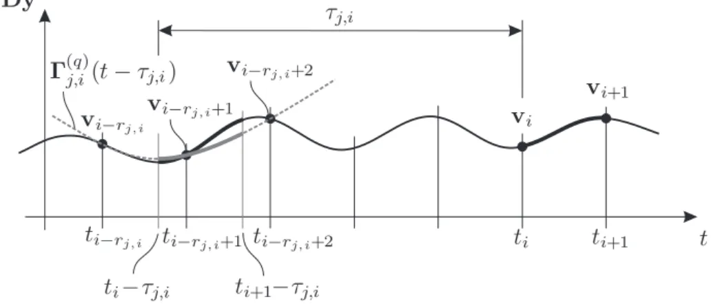
Figure 3.1: Approximation of the delayed term Dy(t − τ_j,i) by the polynomial Γ^(q)_j,i(t−τ_j,i), shown by a dashed line (in the depicted case,q = 2).

where

A_i = 1 h

∫ _t_i+1

ti

A(t) dt , (3.7)

B_j,i = 1 h

∫ _t_i+1

ti

B_j(t) dt , j = 1,2, . . . , g , (3.8) τj,i = 1

h

∫ _t_i+1

ti

τj(t) dt , j = 1,2, . . . , g , (3.9) are the piecewise constant approximations of A(t), B_j(t), and τ_j(t), j = 1,2, . . . , g, over the discretization interval [t_i, t_i+1). Use again the notation y_i := y(t_i) and v_i := v(t_i) for all i ∈ Z. The delayed term Γ^(q)_j,i(t − τ_j,i) is a qth-order Lagrange polynomial interpolation of D(t)y(t) in t ∈ [t_i₋_r_j,i, t_i₋_r_j,i_+q] using the discrete values v_i₋_r_j,i,v_i₋_r_j,i₊₁, . . . ,v_i₋_r_j,i_+q. The integer r_j,i is dened by

r_j,i = int (τ_j,i

h + q 2

)

, j = 1,2, . . . , g , i= 1,2, . . . , p , (3.10) whereintdenotes the integer-part function. The concept of the approximation scheme is illustrated in Figure 3.1, where the dashed curve indicates the approximating poly- nomialΓ^(q)_j,i(t−τ_j,i).

The key feature of the semi-discretization method is that the approximate system (3.4)(3.6) can be solved analytically over the discretization interval t ∈ [t_i, t_i+1) for given initial valuesy_i and v_i+k₋_r_j,i, k= 0,1, . . . , q, j = 1,2, . . . , g, in the form

y_i+1 =P_iy_i+

∑g j=1

∑q k=0

R_j,i,kv_i+k₋_r_j,i , (3.11)

(22)

where

P_i = e^Aⁱ^h , (3.12)

R_j,i,k =

∫ _t_i+1

ti

e^Aⁱ^(tⁱ⁺¹⁻^s) ( _q

∏

l=0, l̸=k

s−τ_j,i−(i+l−r_j,i)h (k−l)h

)

B_j,i ds

=

∫ h 0

e^Aⁱ^(h−s) ( _q

∏

l=0, l̸=k

s−τj,i−(l−rj,i)h (k−l)h

)

B_j,ids (3.13)

(see the variation of constants formula (A.15) in Appendix A). Equations (3.11) and (3.6) imply the discrete map

z_i+1=G_iz_i, (3.14)

where

z_i = (

y_i v_i₋₁ v_i₋₂ . . . v_i₋_r )T

(3.15) is an augmented state vector and the coecient matrix reads

G_i =







P_i 0 · · · 0 0 D 0 · · · 0 0 0 I · · · 0 0

... ... ...

0 0 · · · I 0







(3.16)

+

∑g j=1







0 0 · · · 0 R_j,i,q · · · R_j,i,0 0 · · · 0 0 0 · · · 0 0 · · · 0 0 · · · 0 0 0 · · · 0 0 · · · 0 0 · · · 0

... ... ... ... ... ... ...

0 0 · · · 0 0 · · · 0 0 · · · 0





 .

1 rj,i−q rj,i r

This is an(n+rm)×(n+rm)matrix, wherer = max( r_j,i)

. MatrixG_i can be divided into four blocks, as shown by the lines in (3.16). The left upper block is the n×n matrix P_i. The right upper block consists of r pieces of n×m matrices numbered in (3.16). Matrices R_j,i,k, k = 0,1, . . . , q, are located at the (r_j,i−k)th place within this block. The left lower block of G_i consists of r pieces of m×n matrices (D and zero matrices). The right lower block is an rm×rm block containing zero matrices and identity matrices Iof size m×m.

Utilizing that T =ph, p repeated applications of (3.14) with initial state z₀ gives the monodromy mapping

zp =Φz0 , (3.17)

(23)

where

Φ=G_p₋₁G_p₋₂· · ·G₀ (3.18) is an(n+rm)-dimensional matrix representation of the monodromy operator of (3.4) (3.6), which is at the same time a nite-dimensional approximation of the innite- dimensional monodromy operator of the original system (3.1)(3.2). If all the eigenvalues of Φ are inside the unit circle of the complex plane, then the approximate system (3.4)(3.6) is asymptotically stable. Since discretization techniques preserve asymptotic stability for DDEs (see [75, 63, 84]), the stability charts of the approximate system (3.4)(3.6) give an approximation for the stability charts of the original time-periodic DDE (3.1)(3.2).

The approximation parameter p is related to the resolution of the principal period such thatT =ph; therefore, the integerpis called the period resolution. The integerr is related to the discretization of the state x_t over the delay interval[−τ_max,0], where τ_max = max(

τ_j,i)

, such that τ_max ≈ (r−q/2)h. Therefore, the integer r is called the delay resolution. The number of matricesGi to be multiplied to obtain the monodromy matrixΦin (3.18) is equal to the period resolutionp. The size of the matricesG_i (and the size of the monodromy matrixΦ) is equal to (n+rm). Recall that r= max(

r_j,i) , j = 1,2, . . . , g, i = 1,2, . . . , p, and r_j,i = int(

τ_j,i/h+q/2)

= int(

pτ_j,i/T +q/2)

. Here, r_j,i is the particular delay resolution associated with the particular delay τ_j,i. Thus, the larger the period resolution p, the larger the size of the approximate monodromy matrix. Ifptends to innity, thenΦconverges to the innite-dimensional monodromy operator of the original system (3.1)(3.2).

The convergence of the semi-discretization method can be visualized by plotting the characteristic multipliers in the complex plane. Let us denote the characteristic multipliers of the original system (3.1)(3.2) byµ_k,k = 1,2, . . ., and the characteristic multipliers of the approximate semi-discrete system (3.4)(3.6) byµ˜_k,k= 1,2, . . . ,(n+

rm). Let the circles of center µ˜_k and radius ε be denoted by S_µ_˜_k_,ε. For any small ε >0, there exists an integer M(ε) such that for every p > M(ε), the set ∪n+rm

k=1 S_µ_˜_k_,ε contains exactly n+rm characteristic multipliers µ_k of (3.1)(3.2), and all the other characteristic multipliers have modulus less thanε.

Thus, if all the characteristic multipliers of (3.4)(3.6) have modulus less than 1, then by choosing ε = ¹₂(

1−max_j|µ˜_j|)

, the nite approximation number M(ε) exists, and if p > M(ε), then the discretized system and the original system have the same stability properties (see Figure 3.2 withn+rm= 5).

During the construction of stability charts, the numerical eciency of the method depends, of course, on the choice of the period resolutionp. A lower estimate can be given based on the above derivation ofM(ε), but in practice, it is easier to use a trial- and-error technique and to check how the stability boundaries converge for increasing

(24)

Figure 3.2: Locations of the exact (µ) and the approximate (µ˜) characteristic multipliers.

p. The value of the required pdepends on the system's parameters, which means that the construction of the stability charts can be optimized by choosing dierent values in dierent domains of the charts.

The formulas presented in this section give the steps of the semi-discretization method for arbitrary approximation orderq. For the sake of completeness, some special cases of these formulas are presented for the zeroth- and the rst-order approximations in the next sections.

3.2 Zeroth-Order Semi-Discretization

For the zeroth-order case (q = 0), (3.5) and (3.10) give Γ^(q)_j,i(t−τj,i) ≡ v(ti−rj,i) and r_j,i = int(

τ_j,i/h)

, and the approximate system reads

˙

y(t) =A_iy(t) +

∑g j=1

B_j,iv(t_i₋_r_j,i), t∈[t_i, t_i+1), (3.19)

v(t_i) =Dy(t_i). (3.20)

This corresponds to a piecewise constant approximation of the delayed term according to Figure 3.3.

Using the notation y_i :=y(t_i)and v_i :=v(t_i), i∈Z, the solution over one discrete

(25)

Figure 3.3: Zeroth-order approximation of the delayed term Dy(t − τ_j,i) by Γ⁽⁰⁾_j,i(t−τ_j,i)≡v_i₋_r_j,i, shown by the dashed line.

step can be formulated as

y_i+1 =P_iy_i+

∑g j=1

R_j,i,0v_i₋_r_j,i , (3.21)

whereP_i is given by (3.12) and Rj,i,0 =

∫ h 0

e^Aⁱ^(h⁻^s)dsBj,i. (3.22) IfA⁻_i ¹ exists, then integration gives

R_j,i,0 =(

e^Aⁱ^h−I)

A⁻_i ¹B_j,i , (3.23)

where I is the n×n identity matrix. In this case, the coecient matrix G_i in (3.14) reads

G_i =







P_i 0 · · · 0 0 D 0 · · · 0 0 0 I · · · 0 0

... ... ...

0 0 · · · I 0





 +

∑g j=1







0 0 · · · 0 R_j,i,0 0 · · · 0 0 0 · · · 0 0 0 · · · 0 0 0 · · · 0 0 0 · · · 0 ... ... ... ... ... ...

0 0 · · · 0 0 0 · · · 0





 .

(3.24)

1 rj,i r

Here, matrix R_j,i,0 is located at the r_j,ith place within the right upper block of G_i. The approximate monodromy matrix is given by (3.18).

(26)

3.3 First-Order Semi-Discretization

For the rst-order case(q = 1), (3.5) and (3.10) give

Γ⁽¹⁾_j,i(t−τj,i) =βj,i,0(t)v(ti−rj,i) +βj,i,1(t)v(ti−rj,i+1) (3.25) with

βj,i,0(t) = τ_j,i+ (i−r_j,i+ 1)h−t

h , βj,i,1(t) = t−(i−r_j,i)h−τ_j,i

h , (3.26)

and r_j,i= int(

τ_j,i/h+ 1/2)

. In this case, the approximate system reads y(t) =˙ Aiy(t) +

∑g j=1

Bj,i

(βj,i,0(t)v(ti−rj,i) +βj,i,1(t)v(ti−rj,i+1))

, t∈[ti, ti+1), (3.27)

v(ti) =Dy(ti). (3.28)

The scheme of the rst-order approximation is shown in Figure 3.4. Using the notation y_i :=y(t_i)andv_i :=v(t_i),i∈Z, the solution over one discrete step can be formulated as

y_i+1=P_iy_i+

∑g j=1

(R_j,i,0v_i₋_r_j,i+R_j,i,1v_i₋_r_j,i₊₁)