Modelling and stability analysis of a longitudinal wheel dynamics control loop with feedback delay

(1)

Adam Horvath^a, Peter Beda^a and Denes Takacs^b

aBudapest University of Technology and Economics, Muegyetem rkp. 3, Budapest, HU;

bMTA-BME Research Group on Dynamics of Machines and Vehicles, Budapest, HU

ARTICLE HISTORY Compiled February 16, 2021

CONTACT Adam Horvath. Email: horvath.adam@edu.bme.hu

(2)

ABSTRACT

Vehicle safety is an important field of today’s engineering practice and the scientific research as well. One of the basics of the modern vehicle system dynamics control systems is braking or driving torque control. Ensuring proper connection between the tyre and the road surface is essential for safety and good handling behaviour.

Fundamental questions may arise about the details of the model, such as feedback delay, sampling effect, numerical differentiation in the control algorithm or the dynamical characteristics of the tyre model. In this article a connected dynamical system is presented which contains a wheel model and a PID type traction controller.

Steady state and dynamical brush type tyre models are presented and compared.

Two different ways are described to model the feedback delay. The fully continuous time model contains constant time delay, while there is another case, where the sampling effect and the numerical differentiation methods of the control algorithm are presented. Finally, stability analysis of the delayed system is performed. The stability and performance characteristics and different bifurcations are presented using stability charts. The type of the tyre model has significant effect on the stability characteristics.

KEYWORDS

Active safety; Stability analysis; Tyre dynamics; Control; Vehicle safety

1. Introduction

One of the largest industry where safety critical control systems appear is transporta- tion. Every year new vehicle control functions are developed for passenger cars and commercial vehicles as well. Nowadays, evolution of technology requires more and more precise and efficiently operating solutions. Therefore, detailed and accurate development, analysis and mathematical modelling are becoming more and more important, especially in case of different safety critical control systems. The main goal of the present study is to show up some of the questions of accurate modelling of vehicle dynamics control systems, like dynamic behaviour of tyre models, modelling of time delay and sampling phenomenon, and finally, numerical differentiation methods in the control algorithm. In addition, the effect of these issues on system stability will be treated.

As a ground vehicle is rolling, it is in contact with the environment through wheels and tyres. The tyre forces are generated by the contact between the tyres and the road.

These forces determine the path on which the vehicle is travelling. Proper modelling of this contact is a challenging task. Therefore, there are a huge amount of tyre models for different applications. The theory of tyre modelling is widely discussed in [1]. Dynamic tyre models (e.g. [2], [3], [4], [5], [6], [7]) are used when transient phenomenons are examined, like wheel shimmy or a braking situation with ABS control. But there are cases, when much simpler steady state tyre models (e.g. [8]) are used for dynamic analysis of vehicles or advanced control design, even if steady state models do not contain any detail of the dynamic behaviour of the tyre itself.

Control systems suffer from an effect which has significant influence over the behaviour of the operation, called feedback delay. These delayed control systems are often described with continuous time models, even if the real system contains a digital controller. Delay differential equations (DDE) are widely used as a mathematical model for such systems, as it is presented in [9]. The theory of different types of DDEs are discussed in [10], [11] and [12]. Several methods of stability investigations are presented as well, like Pontriagin’s and Chebotarev’s theorem (see [10] page 53.) or method of D-subdivision (see [10] page 55.). These methods are based on the in- vestigation of the characteristic function of the system. Semi-discretization (see [13])

(3)

provides a numerical method to obtain the stability of DDEs.

There are cases, when continuous time models are unable to describe the feedback loop precisely. For instance, DDEs of advanced type can appear, as it is presented in [14] and [15]. It may be seen, in case of such systems the causality is violated, that leads to instability. As it will be seen later, a controller can be easily made that leads to such a system. Nonetheless, when that control strategy is implemented to a digital system, it can produce well and stable operation. It means, there might be effects that should be considered to make the mathematical model of the system more precise. For instance, one of these effects is sampling.

After considering the effect of sampling, continuous time system will be transformed to a hybrid system. Such a system contains a discrete time part, the digital controller itself, and a continuous time part, that can be a mechanical system as the plant. Semi- discretization may be used to obtain the stability of the hybrid system, as it will be presented. Moving on the details, in digital systems numerical differentiation methods are used to obtain the time derivative of different signals. It means, additional mod- ifications may be necessary regarding the mathematical model. In this research two- point backward-difference formula (BWD) (see [16] page 244.) and high-gain observer (HGO) are used for numerical time-differentiation. Concerning high-gain observers in control applications, [17] presents the basic theory, while [18] describes a derivative tracker based on high-gain observers, and presents the discrete time implementation of it. As an advanced method, [19] presents a switched-gain application of the derivative tracker, that can produce better noise filtering ability.

These issues will be investigated using a wheel traction control system as an example. The article is organized as follows: Section 2 contains the description of the continuous time dynamical model of the control loop. Firstly, the equations of motion of the wheel is presented, that is followed by the dynamic and steady state brush tyre models. Finally, a PID controller and the feedback delay is presented. Section 3 deals with the hybrid model of the control loop, in which sampling and different methods of numerical differentiation are considered. Stability analysis is performed using the method of semi-discretization. Section 4 contains the results concerning the stability maps and performance of the control loop, and some numerical simulation results.

Finally, section 5 is about the conclusions of the study.

2. Continuous time model of the control loop

In this section the continuous time model of the control loop is described. Firstly, the wheel model is shown using the dynamical and the steady state brush tyre model.

Thereafter, the control strategy and the continuous time controller is shown considering feedback delay.

2.1. Equations of motion of the wheel

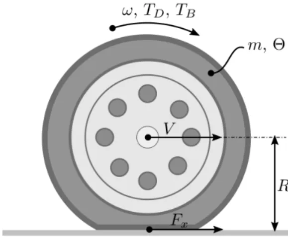
The hereby used wheel model consists of a rotating rigid body and a tyre model which defines the connection between the wheel and the road surface. In this section equations of motion of the rotating rigid body are described, while the tyre model is presented in the next ones. Figure 1 depicts the wheel itself, state variables, external forces and torques and finally the effective radius of the wheel. The state variables are velocity V of the centre point and angular velocity ω. Two separate torques affects the wheel, torque of the transmission is denoted by TD, while braking torque which

(4)

produced by the brake system is denoted byTB. Fx stands for the longitudinal tyre force, which is determined by the tyre model.m denotes the mass, while θ stands for the moment of inertia of the wheel.

Figure 1. Sketch of the wheel with the main parameters, forces and torques

Equations of motion can be obtained with use of Newton’s second axiom. After summarizing external forces and torques equations of motion can be written as

V˙ =Fx

m , (1a)

˙ ω =T_D

θ +T_B

θ −RFx

θ . (1b)

2.2. Dynamic brush tyre model

There are a huge amount of tyre models in the literature, as [1] describes some of the steady state and transient models as well. Modelling the contact between different bodies precisely is a challenging task. In addition, the tyre itself is a complex part of a vehicle, as a composite element it contains different materials and structures.

Therefore, almost every application necessitates a tyre model which is optimised for the special conditions and needs. For the present research it is important to use a physical model, in addition the spatial extent of the contact area between the tyre and the road surface should be considered at least in one dimension. As it is noted in [1], the finite length of the contact patch may be neglected in case of relatively low frequency and large-wavelength transients. Regarding the present application and goal, namely the accurate modelling and stability analysis of the controlled wheel, high frequency transients are assumed as well.

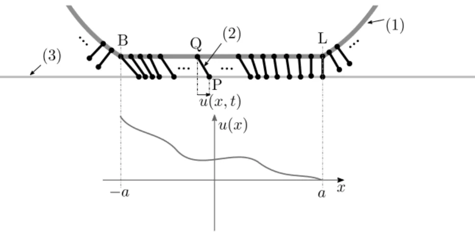
The deformation of the tire is described by means of the brush model (see [1]). This model is built up of massless, infinitesimally small elastic bristle elements which stick to the road surface on a contact line. Figure 2 depicts the sketch of the model. Each of the bristle elements has a point which is connected to the rim – point Q –, and another point which sticks to the road – point P – on the 2a long contact segment.

Leading and back points of this segment are denoted by L and B, respectively. As the wheel rolls, all of the elements moves and rotates with the edge of the rim, therefore an element enters to the segment when reach point L, moves through it, then exits after

(5)

Figure 2. Brush tyre model and the function of deformation. (1) – rim, (2) – a brush element, (3) – road surface

passing through point B. The bristle elements do not effect each other, consequently their deformation can be assumed to be zero outside the contact area.

The principle assumption of this model is that the bristle elements stick to the road surface between points L and B. Furthermore, it means that no sliding effect is modelled regarding the contact between the tire and the road. This assumption can be acceptable in some circumstances, where the force that is generated by the contact is assumed to be small enough. Between the leading and rear points displacement of elements is described by state variableu(x, t), x∈[−a, a], t∈[0,∞).

The kinematic constraint can be derived from the above mentioned principle assumption, namely, that pointP of an element sticks to the road, that is, the velocity of this point is zero with respect to the road surface. Velocity of pointP can be written in form

VP =V(t)−Rω(t)

| {z }

=VQ(t)

+

=_dt^du(x,t)

z }| {

∂

∂tu(x, t)

| {z }

= ˙u(x,t)

− ∂

∂xu(x, t)

| {z }

=u⁰(x,t)

Rω(t) = 0, (2)

which after rearranging can be written as

˙

u(x, t) =Rω(t)−V(t) +u⁰(x, t)Rω(t). (3) Now one can see that the here presented tyre model is of infinite degree of freedom continuum model which is described by partial differential equation (3).

A boundary condition is needed, which is determined by the value of deformation at the leading edge. Outside of the contact segment the deformation is assumed to be zero which implies that the deformation is just zero at pointL. This leads to the Dirichlet boundary condition

u(a, t) = 0, t∈[0,∞). (4)

The contact force consists of elastic and damping effects of the bristle elements.

As one of them is moving from point L to point B, deformation of it is increasing

(6)

continuously, thus the force – which is generated by this element – is increasing, too.

Homogeneity of stiffness and damping coefficients (k and b, respectively) is assumed, that is, same coefficients are considered for all of the elements. The contact force of the whole segment is obtained by the sum of the forces of the brush elements. As the model is a continuum model the contact force can be given as

F_x=k Z a

−a

u(x, t)dx+b Z a

−a

d dtu(x, t)

| {z }

=Rω(t)−V(t)

dx . (5)

For further investigations it is useful to perform a spatial discretization of the continuum model. For this, the contact segment should be divided to N finite intervals, which implies thatN+ 1 brush elements are taken into consideration. Therefore in eq.

(5), integral of the continuous deformationu(x, t) over spatial domain becomes the sum ofN+ 1 trapezoidal area defined by discrete deformation valuesui(t), i= 1. . . N+ 1.

Thus, the longitudinal force can be written in form Fx =k2a

N

N+1

X

i=1

ui(t) +b2a Rω(t)−V(t)

. (6)

Spatial discretization affects not only the longitudinal force, but the governing equation of the model too. The discrete model is governed by N + 1 ordinary differential equations instead of a partial differential equation, and these ODEs can be derived from eq. (3). Firstly, u⁰(x, t) term is approximated with a finite difference formula, then governing equation ofith bristle element reads

˙

u_i(t) =Rω(t)−V(t) +ui−1(t)−u_i(t)

2a N+1

Rω(t), i= 2. . . N + 1, (7) while in case ofi= 1, taking into consideration eq. (4),u1(t) = 0. Finally, the equations of motion of the wheel model can be written as

V˙(t) =2ak mN

N+1

X

i=1

ui(t) +2ab

m Rω(t)−V(t)

, (8a)

˙

ω(t) =TD(t) +TB(t)

θ − 2akR

θN

N+1

X

i=1

ui(t)− 2abR

θ Rω(t)−V(t)

, (8b)

˙

u1(t) =0, (8c)

˙

ui(t) =Rω(t)−V(t) +ui−1(t)−ui(t)

2a N+1

Rω(t), i= 2. . . N + 1. (8d) System of equations (8) contains the equations of the rigid body (1), and equations of the hereby presented tyre model. All of them are autonomous ordinary differential equations. Except for (8d), they are all linear, except for (8b), they are all homogenous.

(7)

2.3. Steady state brush tyre model

In general, steady state models are less computationally intensive compared to the transient or dynamic models.

In perspective of the mathematical model, in case of the dynamic brush model (3) which describes the deformation of the bristle elements is a differential equation, in contrast, in case of the steady state brush model it will be seen that the deformation is determined by an algebraic equation. This fact implies that steady state models are unable to handle the dynamic behaviour of the tyre, nonetheless, steady state models are often use for tasks where strongly dynamic effects rise up.

In the present study, a brush type steady state tyre model will be applied and compared to the dynamic one. The model is presented in [1]. The basic considerations are the same as for the dynamic brush model. As it can be seen in Figure 2, the model consists of elastic bristle elements, and the end of them (point P) sticks to the road surface. While in case of the dynamical model the function of deformation (Figure 2) is a general function over the interval [−a, a], in case of the steady state brush model this function (see (10)) is linear. In addition, relying on [1] it can be seen that the slope of this linear characteristic is the wheel slip itself, that can be written as

κ= V −Rω

V . (9)

With (9) the function of deformation can be written as

u(x) = (a−x)κ . (10)

Integrating (10) over the interval [−a, a], the longitudinal force that is generated by the contact between the tyre and the road can be described as

Fx= 2ka²κ . (11)

Compared to the dynamic brush model, (11) does not contain the term of dissipative effect, and the model is described by a non-linear algebraic formula of the state variablesV andω. The dissipative term could be added to the formula. Using (6), the tyre force can be formulated as

Fx= 2ka²κ+b2a Rω(t)−V(t)

. (12)

2.4. Continuous model of the control system

As it was mentioned in the introduction, here a traction control strategy is used as an example to investigate system stability and performance. The main aim of a traction control is to prevent the wheel from spinning on slippery surface. Therefore, there are cases when it becomes necessary to increase the braking torque to help the wheel to transmit enough traction force. In the present research a simple PID scheme is applied as the basis of the controller. As it can be read in [20], there are two main approaches how the brake force may be controlled by a simple PID controller: wheel slip control and wheel angular deceleration or angular acceleration control. In this research these strategies are used, but instead of slip (see (9)) control angular velocity control is applied, so angular velocity ω(t) and its first time-derivative, angular acceleration

(8)

˙

ω(t) are used as reference signals of the controller. Angular velocity has been chosen instead of wheel slip because the effect of the numerical differentiation can be presented in a more spectacular way if angular velocity and angular acceleration are used.

Let error signale(t) be the difference between a desired set-point and the controlled process variable. Then the mathematical form of the PID controller reads

T_B(t) =k_Pe(t) +k_I Z t

0

e(T)dT +k_De(t)˙ , (13) wherekP,kI, andkD are the coefficients of proportional, integral and derivative terms, respectively.

Velocity of information spread is a non-zero finite value in feedback control systems as well as almost everywhere in the world, therefore, time delay should be considered in the feedback signal. Modelling this effect influences the fundamentals of the model. Until this point of the research, governing equations were ordinary differential equations (system of equations (8)), but after considering feedback delay, a DDE will appear. Fundamentals and stability theory of DDEs with some illustrative examples are described in [10], [11] and [12].

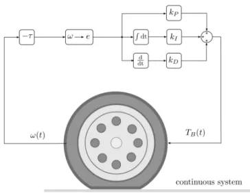
Figure 3.Continuous time coupled dynamical system of the wheel and the PID controller

Considering feedback delay, the brake torque can be given as T_B(t) =k_Pe(t−τ) +k_I

Z t−τ 0

e(T)dT +k_De(t˙ −τ), (14) where τ is the value of the delay. The system which consists of the wheel and the presented controller is depicted by Figure 3. As it can be seen, the physical signal comes from the wheel – here the presence of sensors and signal processing systems, filters etc., as well as actuator dynamics are neglected –, then feedback delay enters, which transformsω(t) toω(t−τ). It is important to note, that here constant delay is

(9)

considered, that is the value of the delay is independent from time.

If the delayed PID control scheme (14) is substituted into the equation of the angular velocity (e.g. (1b)), neutral and advanced types of DDEs are obtained. Firstly, when angular velocity is used for the control, the equation can be written as

˙

ω(t) = k_{P v}

θ (ω_d−ω(t−τ))+k_Iv θ

Z t−τ 0

ω_d−ω(T)dT+k_Dv

θ ω(t−τ˙ )+T_D(t)

θ −RF_x. (15) As it can be seen, the highest order derivative of the delayed term is one, the same as the highest order of the non-delayed term. Therefore (15) implies a neutral system.

In contrast, when angular acceleration is used for the control, the system becomes an advanced type. In this case the equation can be formulated as

˙

ω(t) = kP a

θ ω(t˙ −τ) +kIa

θ Z t−τ

0

˙

ω(T)dT +kDa

θ ω(t¨ −τ) +TD(t)

θ −RFx. (16) Here, subscripts v and a are for velocity and acceleration control, respectively. The delayed term has higher order derivative than the non-delayed term, therefore in this case the causality is violated. This fact implies, that a system that is described with (16) can not be stable. In addition, this equation can not govern a natural system in this form because of the lack of causality.

Nonetheless, a controller, that is used in (16) can be implemented as a digital system, and it results a stable feedback loop.

2.5. Linearization, steady state solution, perturbation

State variables of the system can be divided into two parts. A time independent constant represents a stationary motion

, while a time dependent part represents a small perturbation

e(t)

of the state variable. With these notations, every state variable can be written as the sum of a time independent steady state part and a time dependent part:(t) =+e(t).

Firstly, steady state solution should be determined, the stability will be examined later. The steady state solution can be determined by V or ω, as if free rolling is considered,V =Rω. Obviously, in this case the deformation of each brush element is zero, soui = 0,i= 1. . . N+ 1.

Taking into consideration the steady state solution and the time dependent part and substituting them into (8), equations of the perturbed system can be obtained.

After rearrangements it can be read as

˙

Ve(t) =2ak mN

N+1

X

i=1

eui(t) +2ab

m Rω(t)e −Ve(t)

, (17a)

˙

ω(t) =e T_D

θ +Te_B(t)

θ −2akR θN

N+1

X

i=1

ue_i(t)−2abR

θ Reω(t)−Ve(t)

, (17b)

˙

uei(t) =Rω(t)e −Ve(t) +uei−1(t)−eui(t)

2a N+1

Rω(t), i= 2. . . N + 1. (17c)

(10)

As it may be seen, equation (17c) contains a nonlinear term, in form ui−1(t)−ui(t)

2a

N+1Rω(t) .

After considering small perturbation this nonlinear term can be assumed to be small in second order, so it can be considered to be zero.

In case of the steady state model the linearized form of the wheel slip should be written. Linearizing around the steady state solution, the wheel slip can be written as

κ_lin = ∂κ

∂V

V=V ,ω=ωV(t) +∂κ

∂ω

V=V ,ω=ωω(t) = Rω V²

V(t) + R

Vω(t). (18) 3. Hybrid modelling and stability analysis

As it was described in the previous section, if continuous models are used for the feedback loop, neutral and advanced types of DDEs with constant time delay describe the system. In this section it will be shown, if sampling and numerical differentiation methods are taken into account, the mathematical model becomes a periodic DDE, and the stability of the system can be examined with the method of semi-discretization described in [13].

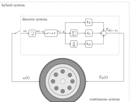
Figure 4. Hybrid model of the wheel and the controller

First of all, the exact meaning of phrase ’hybrid model’ should be unfolded. Figure 4 shows the composition of a digital controller and the continuous wheel model. Until this point of the research, all of the presented parts of the system operates continuously in time domain. Sampling is executed by an analogue-digital converter which is modelled with a zero-order hold that is often comes up in control problems ([18], [13], [21], [20]). Thus, the model can be separated to two main parts. The wheel model can be

(11)

assumed to be a continuous part, while the digital controller is considered discrete in time. These two parts make up the hybrid system.

In addition, there exist industrial applications like vehicle dynamics control systems, where the derivative of a physical signal can not be measured, but it can be calculated by the control algorythm with use of different numerical differentiation methods. That is, such a digital control system does not use the exact derivative of the error signal, for instance ˙e, only the approximated value. Therefore, in case of continuous controllers (see formula (14)), the control signalTB(e,e) depends on both the error signal and the˙ derivative of it as physical signals. In case of a digital implementation, the controller output TB(e) depends on only the error signal, the derivative is calculated from the angular velocity by a numerical method.

3.1. Numerical Differentiation methods

Presenting the discrete part of the model and the numerical methods, firstly discrete time scaleti=ih,i∈Zis introduced, withhas discretization step, or sampling time.

To obtain the first derivative of any signal x(t) with respect to time, finite difference formulas can be used, as it is described in [16]. When real time numerical differentiation is needed, that is, the future values of the signal are unknown, a widespread method that may be used is described by the formula

˙

x(ti)≈ x(ti)−x(ti−1)

h . (19)

It is the formula of the BWD method. Discrete time domain is considered, sot_i is the ith instant of time, and for anyi

t_i−ti−1 =h .

As another approach, HGOs are widely used in nonlinear control. Literature studies a wide range of these problems, like stabilization, regulation, tracking and adaptive control, as it can be seen in [17]. The study provides a well briefing of applications of HGOs, in addition, they introduce the theory of such kind of observers. A method how the time derivatives of a signal can be approximated with an HGO is presented in [18], in addition, this research writes about the discrete time implementation as well.

According to [18] the mathematical model of this derivative tracker observer can be written in form

˙

x(t) =A_dx(t) +H(y_d(t)−C_dx(t)). (20) State vectorx is the vector of estimated derivatives of the input signaly_d,

x(t) =

x(t) x(t)˙ x(t)¨ ... x⁽ⁿ⁾(t)T

.

(12)

System matrixAd is read as

A_d=







0 1 . . . 0 0 0 1 . . . 0

... ...

0 . . . 0 1 0 . . . 0





 ,

while vectorsHand Cd are written in form H=_α₁

α2

² . . . ^αnⁿ

T

,

Cd=

1 0 . . . 0 .

The core of system (20) is estimation error y_d(t)−C_dx(t), that is, multiplied with observer gainH. In H, is a positive small parameter, and constants αi are chosen such that the system is stable. In [22] it is shown using singular perturbation analysis, that after a transient, the estimation error decays toO(), thus the observer can be capable to track the derivative ofy_d accurately.

3.2. Semi-discretization

In contrast to the continuous system, if sampling process is assumed, time delay ap- pears as a periodic function of time. As [13] points out, the latter case may be seen as an approximation of the continuous system. The numerical method described in [13] can be used to describe the hybrid system and using it, stability analysis can be performed. Hereafter, the present study relies on the method described in [13].

Figure 5. Sawthooth-like characteristic of time-periodic delay with different sampling times.h1> h2> h3

For easier understanding, Figure 5 depicts the sawtooth-like characteristic of the periodic delay ρ(t). The input of the digital part of the model is a continuous signal, which is converted to a discrete signal by measuring it at discrete moments. At the instant when a sample is taken, the time delay is exactly (r+ 1)h, then this measured value is constant until the next sample is taken. Between two samples the delay increases from (r+1)hto (r+2)h, then becomes (r+1)hagain, then increases again, and so it goes on. Positive constant r characterize how many samples are delayed in the feedback loop. If a relatively big amount of other sensors and data processing systems

(13)

or data transmitting systems are considered, this value can be high, otherwise it can be assumed to ber= 1. This time-periodic point delay can be described with

ρ(t) = (r+ 1)h+t−ti, t∈[ti, ti+1).

Ifρ(t) is substituted into the continuous perturbed system (17), the resulting equations in general can be written in form

˙

ex(t) =Ax(t) +e Bv(t−ρ(t)), t∈[t_i, t_i+1) (21a)

v(t) =Dex(t), (21b)

where

xe=

Ve(t) eω(t) ue1 . . . ueN+1

contains the state variables of the perturbed system, whilev(t) is the reference signal for the control, andB contains the controller gains. The full system can be separated to two main parts, A represents the wheel, while Bv(t−ρ(t)) contains the formula of the controller with time-periodic point delay presented above. In fact, this delay can be considered as a periodic parametric excitation, therefore (21) is a time-periodic DDE.

For the sake of simplicity, introduce notation (t_i) = i in general for the time signals and state variables. As a result of the delay, in (21) the delayed term remains constant between two periods, therefore (21) can be rewritten as

˙

x(t) =e Aex(t) +Bvi, t∈[ti, ti+1) , (22a)

vi=Dxei, (22b)

Over the interval [ti, ti+1) (22) can be considered as a series of ordinary differential equations with constant forcing, and can be solved. Considering (22), state variable at the instantti+1 can be read as

x_i+1= exp(Ah)

| {z }

=P

x_i+ Z _h

0

exp(A(h−s))dsB

| {z }

=R

vi−r. (23)

Finally, according to [13] (23) and (22b) results the discrete map that can be written in general as





 x_i+1

vi

vi−1

... vi−r+2

vi−r+1







=







P 0 0 . . . R D 0 0 . . . 0

0 1 0 . . . 0 ... . .. ... 0 0 0 . .. 0 0 0 0 . . . 1







| {z }

=G





 x_i vi−1

vi−2

... vi−r+1

vi−r







, (24)

In (24) matrixGrepresents a linear transformation between instantstiandti+1. State

(14)

vectors contain the state variables of the wheel model (xi+1 and xi), and the delayed reference signal samples v_i. . . v_(i−r) for the control. Principal matrix G contains the parameters of the wheel model (in P, as it is marked in (23)), whileR contains the controller gains.

Linear stability analysis can be performed with use of the eigenvalues of the principal matrix. These eigenvalues are called characteristic multipliers of the system. The stationary motion is said to be stable if and only if all the characteristic multipliers have modulus less then one [13]. In other words, if all the characteristic multipliers are located inside the unit circle of the complex plane, the perturbation decays, and after a transient the steady state motion will be set. Otherwise, the system is said to be unstable.

4. Results

The model parameters can be divided into two main groups. One group contains the controller parameters, like sampling time h, the number of delayed samples r and controller gains k_P,k_D, k_I, while one parameter group can be made for the physical parameters of the tyre, namely the half-length of the contact segmenta, stiffnesskand damping coefficient b of the bristle elements. Effect of these parameters on stability will be investigated with use of stability maps. The values of the wheel parameters, sampling time and integral term gain are contained by Table 1. For the results these parameters are used.

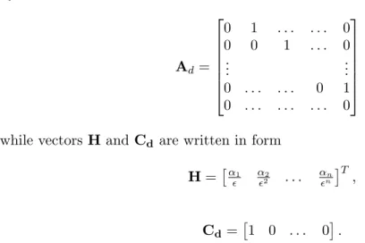
Figure 6. The D-curves of the systems(a)and(b), and the NUE of different parameter domains

For the sake of simplicity, at the beginning of the section new notations are introduced. Angular velocity control with BWD and angular acceleration control with BWD is denoted by(a)and(b), while in case of HGO, the two different control methods are denoted by(c) and(d), respectively. Figure 6 depicts the D-curves (see [11] or [13]) of systems(a)and(b)in the space of proportional and derivative gains. Inside the closed curves the number of unstable eigenvalues (NUE) are shown. Moving through the curves characteristic multipliers are leaving the unit circle. Where a complex pole

(15)

Table 1. Parameters of the wheel model and the controller

Parameter a b k R m Θ h kIv kIa

Value 0.1 1.2·10⁴ 1·10⁷ 1 2500 15 0.05 1000 1000 Unit [m] [Ns/m] [N/m] [m] [kg] [kgm²] [s] [Nm] [Nm/s]

pair has left, Hopf-bifurcation occurs. Where only one pure real pole has left the unit circle, period doubling bifurcation occurs. Where the value of NUE is exactly zero, the system performs stable operation. Where two curves intersect each other double Hopf-bifurcation occurs (denoted by ’HH’ in Figure 6). The characteristic frequency of the solution is shown in this figure for all stability bounds.

If integral gaink_I= 0, the system is said to be stable in the Lyapunov sense, but not asymptotically stable. If asymptotic stability is expected, the integral gain should not be zero, but a positive value. In general it can be said, that high values ofkI reduce the size of the stable area in the stability map with cases(a)and(b)as well. Furthermore, in case(a) with a positive kI Hopf-bifurcation occurs with negative values ofkP. 4.1. Numerical differentiation methods, stable parameter domain and

performance

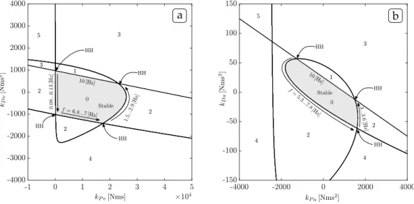
The effect of the two differentiation methods are examined. As it can be seen in Figure 7, in this case the HGO based derivative tracker provides a bigger amount of stable controller gains in contrast with the BWD method. It is important to note, that this increment can be seen only on that parameters which are affected by the differentiation method, in case of type(a) it is only k_Dv, while in case of type(b) all the two parameters are influenced.

Figure 7. Stability maps with different numerical differentiation methods, optimal points are noted by ’+’

and ’x’

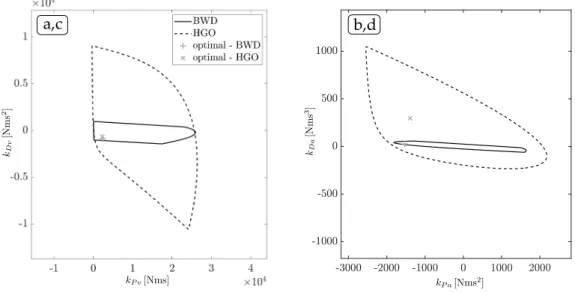
Figure 8 depicts the stable domains, while the grayscale maps represents the distance of the rightmost pole of the system from the imaginary axis, that can characterize the performance of the controller. Here, the two control methods can be compared as well.

(16)

In these cases the angular acceleration control provides better performance, almost two times better as the angular velocity control.

Figure 8. The stable domains, maximum values of Re(λ) and the optimal points denoted by ’+’ and ’x’

As can be seen, the type of the numerical differentiation method doesn’t affect the performance significantly. However, the exact behaviour of the HGO strongly depends on the value of the observer gainH, thus it is possible to influence the performance of the controller with it. It is an important detail, that as it can be seen in Figure 8, negative values of kDv andkP a will provide the best performance for the control.

4.2. Sampling time and the size of the stable domain

Regarding the tyre, the most important parameters are related to the contact between the wheel and the road surface. Stiffness and damping coefficients and the length of the contact segment may affect the system behaviour as they mainly influence the characteristics of the wheel.

(17)

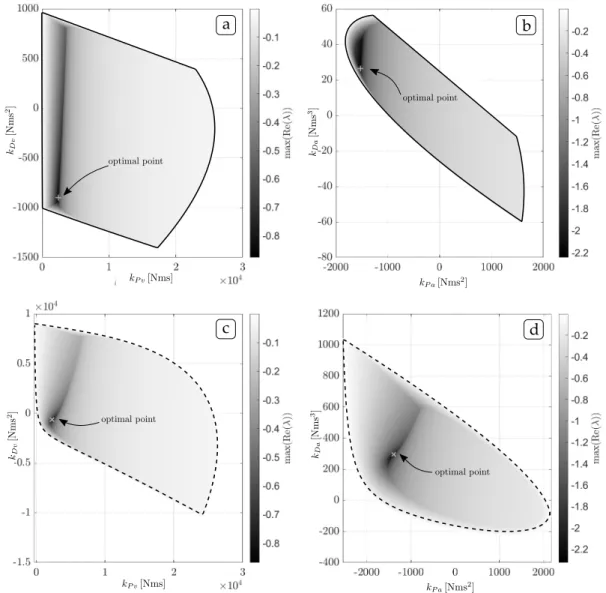
Figure 9. Size of the stable area as a function of the sampling time –a= 0.03 [m],k1 = 10⁶[N/m], k2 = 10⁷[N/m], k3= 5·10⁷[N/m], k4= 10⁸[N/m]

Usually, for controller design tasks wheel and tyre properties are predefined, and only controller parameters can be designed in order to gain a properly functioning system.

Therefore, the attention is drawn to these parameters. Regarding the controller design process one of the most important parameter is sampling timeh. It may be important to know how a change in this parameter affects system stability. In addition, it would be great to know how the tyre parameters and the type of the tyre model itself act the system concerning stability. In the present study two types of brush tyre models are used, and the only and most significant difference between them is the presence of dynamic behaviour.

Figure 9 depicts the size of the stable parameter domain of the angular velocity control as a function of sampling time in case of different stiffness parameters. The curve of the two tyre models can be compared. While in case of the steady state brush model, the size is changing in a ’smooth’ way, in case of the dynamic model there

(18)

Figure 10. Size of the stable area as a function of the sampling time –a= 0.03 [m],k1 = 10⁶[N/m], k2= 10⁷[N/m], k3= 5·10⁷[N/m], k4= 10⁸[N/m]

are changes with much higher gradient. The amount of these changes or so called oscillations in the size of the stable area are growing with the growth of the stiffness value. While in the first case, there are only one local maximum of the solid curve, in the last case there are a huge amount of them. In contrast, the steady state model does not produce these oscillations. In addition, the tendency of the curves of the steady state model is changing with the stiffness value as well. That means, with relatively low stiffness values decreasing of the sampling time may cause instability, while with higher stiffness, the size of the stable area is increasing.

In case of angular acceleration control, in Figure 10, the behaviour of the size transition is almost the same. With lower values of the stiffness the two curves are almost running together, while with high values the oscillations rise up. In this case, the tendency of the curves remain the same. With decreasing sample time the size is decreasing, and there is a value where it is practically zero.

(19)

The presence of the oscillations may be caused by the fast movements of the D curves of the system. These results shows that the steady state model does not contain probably important dynamic effects of the tyre. Although, as it can be seen in Figures 9 and 10, there is a value of the sampling time where the curve of the dynamical model goes close to the curve of the steady state model, and the oscillations disappear. Above this value, the steady state model provides accurate solutions for the stability of the dynamical model. Nonetheless, it is seen that there are modelling tasks where the dynamical behaviour should not be neglected for the sake of accuracy.

It is important to remind the reader, that the continuous model of the angular velocity control is a neutral system, while in case of the angular acceleration control it is an advanced system. Sampling can be considered as a imperfection in continuity, if this imperfection tends to zero, that is, the hybrid system tends to the continuous system, the shape of the stable domain tends to the continuous system’s stable area.

An advanced system can not be stable because of the violated causality, and this can be captured in Figure 10, since the stable domain is shrinking with decreasing sampling time in every cases. But not in case of a neutral system. Regarding Figure 9, the exact behaviour can not be determined, and the impact of a change of the stiffness value can be unpredictable regarding stability.

4.3. Simulation results

Numerical simulation of the full system can be a used to validate the qualitative behaviour of the system. Now, stability stands in focus of the study, and one can determine easily the behaviour of present system regarding stability with use of time domain signal analysis. If time evolution of state variables presents increasing tendency with or without oscillations in the signals, system is considered unstable, but if perturbation decays and steady state value is set, the system can be considered stable.

Now, for simulation Simulinkis used as a development environment, as it provides easy-to-use but powerful techniques to build such kind of hybrid systems. Figure 11 depicts layout of the simulation model.

Figure 11. The Simulinkmodel

The model is divided to two main parts: the controller, which is modelled as a discrete time system and the continuous time model of the wheel. It is important to note, that a numerical simulation can not be a real continuous solution in time, it is only a discrete approximation of it, therefore, for the sake of simplicity, hereinafter the continuous part of the simulation will be referred as quasi-continuous. Between

(20)

the two main parts rate transition blocks are placed, which blocks are responsible for sampling the quasi-continuous output signal of the wheel model with the sample time of the controllerh, and for transforming the controller’s discrete output signal to the wheel model’s quasi-continuous input signal. Controller submodel contains discrete version of equation (14), while the wheel is represented by the equations of (8).

Figure 12 contains four marginally stable simulation results. Each plots contain the step driving torque signal (T_D) with dashed line and the controller output braking torque signal (TB) with solid line. These results shows the difference between the

Figure 12. Marginally stable solutions – semi-discretization and simulation results

different stability boundaries regarding the frequency of the solution. In this case, the maximum frequency isf_max = 10 [Hz]. When the controller gains are located on the bottom or on the top bounds, the main frequency is relatively high, while in case of the right and left bounding curves these frequencies are lower.

Time signals can be captured in Figure 13. Under each other, three diagrams are placed. The first and second diagrams are the velocityV(t) and the angular velocity ω(t) respectively, while the last diagram contains the driving torque signalT_D (with dashed line) and the braking torque signal TB(t). In the first case a stable operation can be captured. As driving torqueT_D(t) rises from 0 to 100, the braking torque sets to the same value. After a transient period, the controller error and the oscillations decay. In the second case, the system is marginally stable. There is a low frequency part of the solution that decays, but a high frequency periodic solution remains. The third part depicts an unstable simulation, where the perturbations do not decay.

5. Conclusions

The presented study has highlighted some important aspects of accurate modelling and analysis of a wheel controller. As it can be seen, there are effects that can cause

(21)

Figure 13. Stable, marginally stable and unstable simulation results

significant change of the main system characteristics.

The type of tyre model has strong effect on stability properties. On the edge of stable operation, strongly dynamic effects appear. Therefore, the steady state brush model can not provide a quite accurate description of the system behaviour. Below a certain value of the sampling time of the digital controller, the dynamical model cause an oscillation on the size of the stable domain, that is, the D-curves are moving fast, while the sampling time is varying. In case of the steady state brush model, this fast changing can not be captured. It means, the steady-state model can be used for approximating the dynamical behaviour of the controlled wheel, especially with relatively large sampling time of the digital system. Nonetheless, the dynamical model provides a more accuracy, the dynamical details should not be neglected with relatively small sampling time.

It has been presented that the presence of feedback delay has a significant effect on the stability properties. First of all, in some cases continuous models can not be used, and sampling needs to be considered, especially in case of advanced type systems.

It is important to note, that considering feedback delay is important because the presence of this time delay implies a different mathematical model, called DDE. These differential equations has some crucial features. It is enough to mention the advanced type system. While in the continuous case the causality is violated, that is, the system can not be stable, the sampling as a parametric excitation can stabilize it. However, in contrast with the non-delayed systems, the stable parameter domain shrinks if the sampling time decreases. In addition, the neutral type system can produce increasing and decreasing characteristics as well, depending on the tyre parameters.

The numerical differentiation technique that is used in the control algorythm affects the characteristics of the system. The simple BWD technique provides an easy and less computationally intensive way to obtain the time derivative of a signal. In contrast, the HGO requires more resources to use and observer gains must be tuned well. The tuning provides an opportunity to affect the size of the stable parameter domain, the exact location of the parameters belonging to the best performance, and the noise filtering characteristics as well. Therefore, an HGO is a versatile application for numerical time differentiation.

Overall, it can be said that dynamical tyre models should be used for stability analysis, and in case of highly dynamic scenarios, as these models contain important details of the wheel as a dynamical system. The feedback delay should be considered during the design process, since neutral and advanced type systems can appear, and

(22)

they have particular stability characteristics. The effect of sampling should be taken into consideration as well, since without it key properties are neglected. Last, but not least, it could be advantageous to use complicated numerical differentiation methods, as they provide an opportunity to affect the stability and performance properties.

Acknowledgements

This work was supported by the National Research, Development, and Innovation Office of Hungary under grant no. NKFI-128422; and the Pro Progressio Foundation.

References

[1] Pacejka HB, Besselink I. Tire and vehicle dynamics. 3rd ed. Amsterdam:

Elsevier/Butterworth-Heinemann; 2012. Engineering Automotive engineering; oCLC:

796260687.

[2] Beregi S, Takacs D, Stepan G. Bifurcation analysis of wheel shimmy with non-smooth effects and time delay in the tyre–ground contact. Nonlinear Dynamics. 2019 Oct;98(1):841–

858. Available from: http://link.springer.com/10.1007/s11071-019-05123-1.

[3] Romano L, Bruzelius F, Jacobson B. Unsteady-state brush theory. Vehicle System Dynamics. 2020 May;:1–29Available from:

https://www.tandfonline.com/doi/full/10.1080/00423114.2020.1774625.

[4] Ran S, Besselink I, Nijmeijer H. Application of nonlinear tyre models to anal- yse shimmy. Vehicle System Dynamics. 2014;52(sup1):387–404. Available from:

https://doi.org/10.1080/00423114.2014.901542.

[5] Ataei M, Khajepour A, Jeon S. Model predictive control for integrated lateral stability, traction/braking control, and rollover prevention of elec- tric vehicles. Vehicle System Dynamics. 2020;58(1):49–73. Available from:

https://doi.org/10.1080/00423114.2019.1585557.

[6] Basrah MS, Siampis E, Velenis E, et al. Wheel slip control with torque blending using linear and nonlinear model predictive control. Vehicle System Dynamics. 2017;55(11):1665–

1685. Available from: https://doi.org/10.1080/00423114.2017.1318212.

[7] Mantripragada VKT, Kumar RK. Sensitivity analysis of tyre characteristic parameters on abs performance. Vehicle System Dynamics. 2020;0(0):1–26. Available from:

https://doi.org/10.1080/00423114.2020.1802491.

[8] Pacejka HB, Bakker E. THE MAGIC FORMULA TYRE MODEL.

Vehicle System Dynamics. 1992 Jan;21(sup001):1–18. Available from:

http://www.tandfonline.com/doi/abs/10.1080/00423119208969994.

[9] Hu H, Wang Z. Dynamics of Controlled Mechanical Systems with Delayed Feedback. Berlin, Heidelberg: Springer Berlin Heidelberg; 2002. Available from:

http://link.springer.com/10.1007/978-3-662-05030-9.

[10] Kolmanovski˘ı VB, Nosov VR. Stability of functional differential equations. London ; Or- lando: Academic Press; 1986. (Mathematics in science and engineering; v. 180).

[11] St´ep´an G. Retarded dynamical systems: Stability and characteristic functions. Longman Scientific & Technical; 1989. Pitman research notes in mathematics series; Available from:

https://books.google.hu/books?id=laFhQgAACAAJ.

[12] Hale JK, Lunel SMV. Introduction to Functional Differential Equations. (Applied Math- ematical Sciences; Vol. 99). New York, NY: Springer New York; 1993. Available from:

[13] Insperger T, St´ep´an G. Semi-Discretization for Time-Delay Systems. (Applied Mathe- matical Sciences; Vol. 178). New York, NY: Springer New York; 2011. Available from:

(23)

[14] Insperger T, Stepan G, Turi J. Delayed feedback of sampled higher derivatives. Philosophical Transactions of the Royal Society A: Mathematical, Phys- ical and Engineering Sciences. 2010 Jan;368(1911):469–482. Available from:

https://royalsocietypublishing.org/doi/10.1098/rsta.2009.0246.

[15] Kovacs BA, Insperger T. Retarded, neutral and advanced differential equation models for balancing using an accelerometer. International Journal of Dynamics and Control. 2018 Jun;6(2):694–706. Available from: http://link.springer.com/10.1007/s40435-017-0331-9.

[16] Sauer T. Numerical analysis. 2nd ed. Boston: Pearson; 2012. OCLC: ocn725295545.

[17] Khalil HK, Praly L. High-gain observers in nonlinear feedback control: HIGH- GAIN OBSERVERS IN NONLINEAR FEEDBACK CONTROL. International Jour- nal of Robust and Nonlinear Control. 2014 Apr;24(6):993–1015. Available from:

http://doi.wiley.com/10.1002/rnc.3051.

[18] Dabroom AM, Khalil HK. Discrete-time implementation of high-gain observers for numerical differentiation. International Journal of Control. 1999 Jan;72(17):1523–1537. Avail- able from: https://www.tandfonline.com/doi/full/10.1080/002071799220029.

[19] Ahrens JH, Khalil HK. High-gain observers in the presence of measurement noise:

A switched-gain approach. Automatica. 2009 Apr;45(4):936–943. Available from:

https://linkinghub.elsevier.com/retrieve/pii/S0005109808005591.

[20] Savaresi SM, Tanelli M. Active braking control systems design for vehicles. London ; New York: Springer Verlag; 2010. Advances in industrial control; oCLC: ocn646113891.

[21] Okuyama Y. Discrete control systems. First edition ed. New York: Springer; 2014. OCLC:

ocn861323253.

[22] Esfandiari F, Khalil HK. Output feedback stabilization of fully linearizable systems. International Journal of Control. 1992 Nov;56(5):1007–1037. Available from:

http://www.tandfonline.com/doi/abs/10.1080/00207179208934355.