On the global dynamics of connected vehicle systems

(1)

https://doi.org/10.1007/s11071-019-04889-8

O R I G I NA L PA P E R

On the global dynamics of connected vehicle systems

Adam K. Kiss · Sergei S. Avedisov · Daniel Bachrathy · Gábor Orosz

Received: 23 November 2018 / Accepted: 13 March 2019

Abstract In this contribution, heterogeneous connected vehicle systems, that include human-driven as well as connected automated vehicles, are investigated.

The reaction time delay of human drivers as well as the communication and actuation delays of connected automated vehicles is incorporated in the model. Satu- rations due to the speed limit and limited acceleration capabilities of the vehicles are also taken into account.

The arising nonlinear delayed system is studied using analytical and numerical bifurcation analysis. Stability analysis is used to identify regions in parameter space where oscillations arise due to loss of linear stability of the equilibrium. Moreover, with the help of numerical continuation, bistability between the equilibrium and oscillations is shown to exist due to the presence of an isola. It is demonstrated that utilizing long-range wire- less vehicle-to-vehicle communication the connected automated vehicle is able to eliminate the oscillations and keep the traffic flow smooth.

Keywords Time delays · Bistability ·Vehicle- to-vehicle (V2V) communication · Connected automated vehicle·Beyond-line-of-sight information· Acceleration saturation

A. K. Kiss (

B

⁾ ^·D. Bachrathy

Department of Applied Mechanics, Budapest University of Technology and Economics, Budapest 1111, Hungary e-mail: kiss_a@mm.bme.hu

S. S. Avedisov·G. Orosz

Department of Mechanical Engineering, University of Michigan, Ann Arbor, MI 48109, USA

1 Introduction

Road transportation is expected to go through a huge transformation in the upcoming decades with the introduction of connected and automated vehicles. While such technologies mainly aim at improving passenger comfort and safety, they may also be used to improve the overall traffic flow. For example, by controlling the motion of automated vehicles may lead to higher traffic throughput and improved fuel economy [1–7].

Most prior research on the topic assumed 100% pene- tration rate of automation as well as vehicle-to-vehicle (V2V) connectivity. While the latter one is expected to rise rapidly in the next few years, the former one will likely follow in a slower pace due to the high cost of these vehicles. Thus, there is a need to understand the dynamics of mixed scenarios where automated vehicles are mixed into the flow of human-driven traffic. Initial research on mixed scenarios typically considered linear dynamics [8–10], while recent experimental results show that nonlinearities may play an important role in these systems [11–13].

In this paper, we start with modeling the longitudinal dynamics of human-driven vehicles. Then, a connected cruise control (CCC) algorithm is proposed to regulate the longitudinal dynamics of connected automated vehicles (CAVs) which utilize motion information from multiple human-driven vehicles ahead (within and beyond the line of sight). In particular, our goal is to design CCC controllers for CAVs so that they can mitigate traffic waves at the linear and nonlin-

(2)

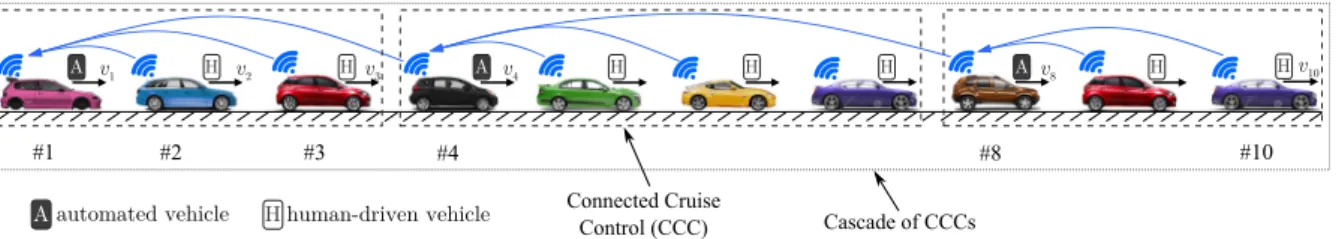
Fig. 1 Schematic representation of vehicles on a single lane. Cascade of CCCs consisting of human-driven and connected automated vehicles. Arrows show the direction of information propagation via V2V communication

ear levels. We adopt the strategy of “do not look ahead of another CAV” leading to the formation of a cascade of CCCs, as depicted in Fig.1. This allows for a modular and scalable design of connected vehicle systems [14]. When modeling the vehicles, we incorporate time delays to represent the human reaction time and the communication and actuation delays of connected automated vehicles. Moreover, we take into account the speed limits and limited acceleration capabilities of vehicles, which introduce nonlinearities into the modeling equations.

In order to select the control gains of the connected automated vehicles, linear and nonlinear analyses are carried out while the vehicles placed on a circular road.

First, linear stability analysis is presented to understand the effects of the connected automated vehicles on the stability of the uniform flow. With the help of the insta- bility gradient method [15], we construct robust stability diagrams in the plane of the control parameters. We demonstrate that using beyond-line-of-sight information (obtained via V2V communication) can improve linear stability. Then, nonlinear analysis is carried out to have an insight into the influence of limited acceleration capabilities of vehicles. We use numerical continuation techniques [16,17], to draw the skeleton of the traffic dynamics as a three-dimensional wire frame representation. For the first time, we demonstrate that acceleration saturation leads to new dynamic behavior, where bistable regions appear through the presence of isolas. In this scenario, no linear stability loss occurs, but larger perturbations may still trigger traffic waves.

Then, the effects of connected automated vehicles are investigated at the nonlinear level. We demonstrate that when using information only from the vehicle immediately ahead, an automated vehicle cannot eliminate the isolas. However, including additional information from beyond-line-of-sight, a connected automated vehicle can make the uniform flow globally stable.

The paper is organized as follows: in Sect. 2, we provide the governing equations of heterogeneous connected vehicle systems (including human-driven and automated vehicles) and explain the sources of the nonlinearities. Section3gives the linear stability analysis for the proposed model. A case study is conducted in Sect.4 with a connected automated and two human- driven vehicles with detailed linear stability analysis.

Then, in Sect.5, we analyze the nonlinear effects of the acceleration saturation using numerical continuation. Finally, in Sect.6, we conclude our results and discuss future directions.

2 Governing equations

In this section, we model the car-following behavior and the corresponding governing equations of heterogeneous connected vehicle systems. We consider that human drivers respond to the motion of the vehicle immediately ahead, while the connected automated vehicle’s connected cruise control algorithm can utilize motion information from up tokcars ahead. We place N vehicles on a ring of length L such that we haveMautomated andN−Mhuman-driven vehicles.

The distribution of the human-driven vehicles and the connected automated vehicles are described with the help of the indices ih ∈ H and ia ∈ A, such that A+H = {1, . . . ,N}and| A| + |H|= N.

Following the models in [18], the governing equations can be given as:

˙ vi = f

α

V(h^σ_i)−v_i^σ +

k_i

j=1

βj

v_i^σ₊_j −v^σ_i

if i =ia, (1)

˙ vi = f

αh

V(h^τ_i)−v_i^τ +βh

v_i^τ₊₁−v_i^τ if i =ih,

(3)

h˙i =vi+1−vi,

where the dot stands for differentiation with respect to timetand we use the abbreviated notationv_i^ϑ =vi(t− ϑ)to indicate delays. Also,vi denotes the velocity of vehiclei andhi denotes the distance headway, that is, the bumper-to-bumper distance between the vehiclei and its predecessor. This can be calculated as

hi =xi+1−xi−li, (2) where xi denotes the position of the rear bumper of vehicleiandlidenotes the length of vehicleisuch that L=_N

i=1(hi+li)is the length of the ring. It should be noted that fori=N, we havehN =L−_N₋₁

i=1 (hi+ li)−lNandvN+j =vjdue to periodicity imposed by the ring. In case of a human-driven vehicle (i = ih), the sum of the reaction time delay and the actuation delay is denoted byτ, while for a connected automated vehicle (i = ia), the sum of the communication and actuation delay is denoted byσ.

The parametersαandβjare the control parameters of the connected automated vehicle, andαhandβhare the control parameters of the human-driven vehicles.

For the sake of simplicity, all human-driven vehicles are considered to be identical and so the automated ones.

Theβ parameters are directly related to the velocity differences, while theαparameters are related to the optimal velocity functionV(h)(also called range policy), that satisfies the following properties:

1. V(h) is continuous, smooth and monotonically increasing (the more sparse the traffic is, the faster the vehicles want to travel).

2. V(h) ≡ 0 for h ≤ hst (in dense traffic vehicles intend to stop).

3. V(h)≡ vmax forh ≥ hgo (in sparse traffic vehicles intend to travel with the maximum speed, also called free-flow speed)

These properties can be summarized as:

V(h)=

⎧⎨

⎩

0 if h≤hst, F(h) if hst<h<hgo, vmax if h≥hgo,

(3)

where F(h) is strictly monotonically increasing and satisfiesF(hst)=0 andF(hgo)=vmax. In this paper,

(a) (b)

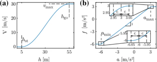
Fig. 2 Source of the nonlinearities in the model:asaturations due to the speed limit in the range policy function (4);baccelera- tion saturation function (6). The parameters area_min= −6 m/s², a_max=3 m/s²,c=0.05 m/s²

Fig. 3 A simple CCC placed on a ring where the first car is automated and the second and third cars are human driven (N= 3,M=1)

we present the results using the range policy function

F(h)= vmax

2

1−cos

π h−hst

hgo−hst

, (4)

that is smooth athstandhgo; see Fig.2a. For simplicity, we use the sameV(h)function for human-driven and automated vehicles.

Saturations due to limited acceleration capabilities of vehicles are also taken into account by the function

f(a)=

⎧⎨

⎩

amin if a <amin, a if amin≤a≤amax,

amax if a >amax, (5) whereaminandamaxare the lower and upper saturation bounds, respectively.

However, the nonsmoothness ataminandamaxmay lead to computational challenges. In order to avoid these, we smooth the saturation function by introduc- ing a smoothness range, where the different sections defined in Eq. (5) are connected to each others while

(4)

Table 1 Parameters in the

test case Total veh. numb.N 3 max. speedvmax 30 m/s

CCC veh. numb.M 1 Stop dist.h_st 5 m

Human delayτ 1 s Driving dist.h_go 55 m

CCC delayσ 0.5 s Lower satur. limita_min −6 m/s²

Human gainαh 0.2 1/s Upper satur. limita_max 3 m/s²

Human gainβh 0.4 1/s Smoothness rangec 0.05 m/s²

maintaining Cⁿcontinuity. In particular, to maintain C¹ continuity, we use second-order polynomials, yielding

f(a)=

⎧⎪

⎪⎪

⎨

⎪⎪

⎪⎩

amin if a≤amin−c,

a+^(a^min^−a+c)_4c ² if a_min−c<a<a_min+c, a if amin+c≤a≤amax−c, a−^(a^max^−a−c)_4c ² if amax−c<a<amax+c, amax if a≥amax+c.

(6) Additional parameters can be found in Table1.

3 Linear stability analysis

In this section, we present the mathematical back- ground of the linear stability analysis of the connected vehicle system. Setting the left-hand side of Eq. (1) to be zero, we obtain the unique equilibrium:

vi(t)≡v^∗=V(h^∗),

hi(t)≡h^∗=L/N, (7)

where vehicles travel with constant speed while keep- ing constant distance. Using the vector

x(t)=

v1(t)· · ·vN(t)h1(t)· · ·hN(t)T

, (8)

the equilibrium can be given as x^∗=

v^∗· · ·v^∗h^∗· · ·h^∗T

. (9)

Substituting the perturbationy(t)=x(t)−x^∗into Eq. (1), using a Taylor series expansion and dropping the higher-order terms, we obtain the variational system

˙

y(t)=Ly(t)+Py(t−τ)+Ry(t−σ ). (10)

The 2N×2Ncoefficient matrix in front of the non- delayed term is given by

L=

0 0 S−I 0

, (11)

whereIstands for theN×N identity matrix andSis anN×Ncirculant matrix, defined as

S=

⎡

⎢⎢

⎢⎣

0 1 0 . . .0 ... ... ...0

0 1

1 0. . . 0

⎤

⎥⎥

⎥⎦. (12)

The 2N ×2N coefficient matricesP andRin front of the delayed terms correspond to the human-driven vehicles and the automated vehicles, respectively. In particular, we have

P= −H

(αh+βh)I+βhS

αhκH

0 0

, (13)

whereκ =V(h^∗)is the gradient of the range policy function at the equilibrium. Also note that atx^∗, the saturation function gives f(0)=1. TheN×Nindicator matrixHcontains zero elements except those diagonal terms which correspond to human-driven vehicles, that is,

Hi,i =

1 if i =ih,

0 if i=ia. (14)

Moreover, we have

R=

−(I−H) (α+k

j=1βj)I+k j=1βjS^j

ακ(I−H)

0 0

,

(15)

(5)

where(I−H)corresponds to the automated vehicles.

In order to determine the stability of the equilibrium, we utilize the D-subdivision method [19–21]. Substi- tuting the trial functiony(t)=ce^λ^t into Eq. (10), the corresponding characteristic equation becomes D(λ)=det

λI−L−Pe^−λτ −Re^−λσ

=0. (16) The real and the imaginary parts of the characteristic roots are computed using the multi-dimensional bisection method (MDBM), which can find all the roots within a selected domain in the complex plane when using a sufficiently dense initial mesh [22].

The system is stable if all characteristic roots have negative real parts, i.e., Reλi <0 for alli =1,2, . . .. By substitutingλ = iωcr,ωcr ≥ 0 into Eq. (16), the stability boundaries can be determined [19–21].

In case of large number of vehicles, solving Eq. (16) can be time consuming and sensitive for rounding errors. However, in case of special patterns of distribution of the automated vehicles, where every(K = N/M)th vehicle is automated, Eq. (16) takes the ana- lytical form

D= a0b₀^K⁻¹

M

−

(−1)^K⁻¹a2b0b₁^K⁻²+(−1)^Ka1b₁^K⁻¹ M

.(17) Here,M is the number of connected automated cars, each monitoring the motion of K −1 human-driven vehicles ahead, and the coefficients read as

a0=λ

λ+(α+β1+β2)e^−λσ

+ακe^−λσ, b0=λ

λ+(αh+βh)e^−λτ

+αhκe^−λτ, a1= −

λβ1+ακ e^−λσ, b1= −

λβh+αhκ e^−λτ, a2= −λβ2e^−λσ.

(18)

4 Stability analysis of a simple connected vehicle system

In this section, the stability analysis is applied to the simplest case of CCCs with 3 cars on a ring, where the first vehicle is automated, while the second and third cars are human driven (N =3,M =1); see Fig.3.

We analyze the effects of the average headwayh^∗ and the design parameters of the autonomous vehicle

α,β1andβ2, while the other parameters, such as the parameters of the human drivers and the time delays, are kept fixed. The applied parameters together with reaction time delays are presented in Table1, see the related parameter identification techniques in [10,13].

The corresponding coefficient matrices in the lin- earized system (10) read as follows:

L=

⎡

⎢⎢

⎣

0 0 0 0 0 0 0 0 0 0 0 0 0 0 0 0 0 0

−1 1 0 0 0 0 0 −1 1 0 0 0 1 0 −1 0 0 0

⎤

⎥⎥

⎦

, H=

⎡

⎣0 0 0 0 1 0 0 0 1

⎤

⎦. (19)

cf. (11) and (14), while the coefficient matrices of the delayed terms are

P=

⎡

⎢⎢

⎣

0 0 0 0 0 0

0 −(αh+βh) βh 0αhκ 0 βh 0 −(αh+βh)0 0 αhκ

0 0 0 0 0 0

⎤

⎥⎥

⎦ ,

(20) and

R=

⎡

⎢⎢

⎣

−(α+β1+β2) β1β2ακ 0 0

0 0 0 0 0 0

⎤

⎥⎥

⎦

, (21)

cf. (13) and (15).

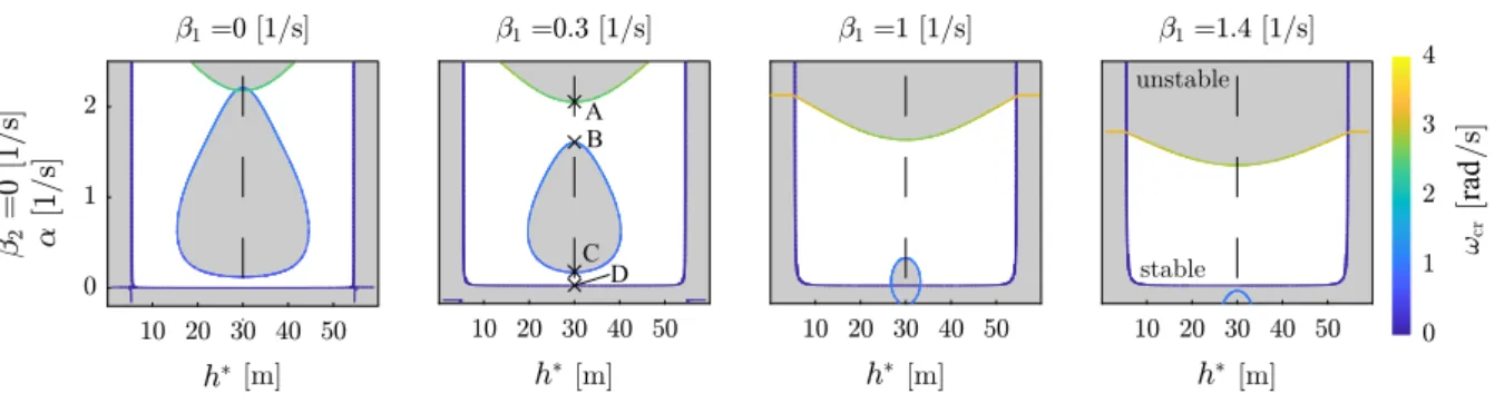
As a first step, we analyze the influence of an automated car that does not utilize beyond-line-of-sight information (β2=0) on the traffic dynamics by draw- ing the stability chart in the plane ofh^∗andαfor differ- entβ1parameters. In the stability charts in Fig.4, the gray areas identify regions in parameter space where oscillations arise due to loss of linear stability of the equilibrium. The coloring of the boundaries shows the frequency of the Hopf bifurcation in the corresponding nonlinear system. The darkest blue corresponds to ωcr = 0, that is related to a fold bifurcation. All the charts show stable range only betweenh^∗ ∈ [5,55]

m. Outside of this domain, the saturation in the range

(6)

Fig. 4 Linear stability diagrams for differentβ1values without beyond-line-of-sight information (β2=0). Gray areas correspond to the linearly unstable parameter combinations, while white areas are linearly stable. The color of the stability boundary

corresponds to the frequency of arising oscillations when stability is lost. Note that the parametersα,β1andβ2correspond to the automated vehicle, while parameters of the human drivers are given in Table1. (Color figure online)

Fig. 5 The effect of theβ1parameter forh^∗=30 m. The white areas are robustly stable for any average headwayh^∗. In the gray area, a stable or an unstable equilibrium may exist depending on the average headwayh^∗

policy function eliminates the headway control so that equilibrium in (7) does not exist. Furthermore, negative αvalues always lead to unstable motion due to positive feedback.

For the leftmost panel in Fig.4(atβ1 =0), large unstable range in the shape of a “droplet” can be found.

This is centered aroundh^∗=30 m, which corresponds to the largest derivative of the range policy function (κ = 0.943 1/s). Comparing the different panels in Fig.4, the unstable droplet is shrinking when increasing parameterβ1. However, the droplet is also shifting downward and merging with the unstable region α <0. Forβ1>1.3 1/s, the droplet is completely van- ished and a large stable area forms. However, such large control parameter may require large acceleration that may not be possible under limited acceleration capabil-

ities. Notice that the upper unstable area is also shifting downward asβ1increases, but only causes instabilities for unrealistically largeαvalues.

We prefer those robust control parameters for which the system is stable for any available headwayh^∗ ∈ [5,55]m. The corresponding stability boundaries can be found by following the edges of the droplets where the tangent is horizontal (ath^∗=30 m in our case) [23].

That is, if we change parameterh^∗, the real parts of the critical characteristic roots remain zero (Reλ=0).

This condition can be described as follows:

Re ∂λ

∂h^∗

=0, (22)

while setting the critical valueλ = iωcr. This can be rewritten as

Re

−^∂

D(λ)

∂h^∗

∂D(λ)

∂λ

=0, (23)

using implicit differentiation of the characteristic equation Eq. (16). Thus, the robust parameter boundaries can be calculated by solving the real and imaginary parts of Eqs. (16) and (23) together while setting λ=iωcr.

In the 4-dimensional parameter space (h^∗, β1, α, ωcr), Eqs. (16) and (23) give us a 1-dimensional object (curve). Still multi-dimensional bisection method can be used to find the corresponding solutions. Figure5 shows the corresponding robust stability boundaries against the variation in the average headwayh^∗in the plane ofβ1andαcontrol parameters, while color indi- cates the critical frequencyωcr. Two robustly stable

(7)

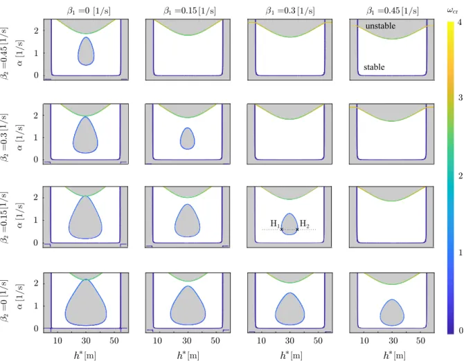
Fig. 6 Linear stability charts for different values ofβ1andβ2. The same notation is used as in Fig.4

Fig. 7 Robust stability diagram in the plane of parametersβ1

andβ2. The same notation is used as in Fig.5except that color represents the critical values ofα

domains can be observed. However, the lower one is not practical as such smallαvalues may not be safe.

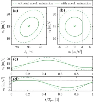
Fig. 8 Bifurcation diagram showing peak-to-peak amplitude of velocity oscillations for the automated vehicle as a function of the average headway. Continuous and dashed curves correspond to the model with and without acceleration saturation, respectively.

The control parameters areβ1 = 0.3 1/s,β2 = 0.15 1/s and α=0.6 1/s. (Color figure online)

When the connected automated vehicle can utilize beyond-line-of-sight information (with nonzero

(8)

(a) (b)

(c)

(d)

Fig. 9 Periodic orbits with acceleration saturation (continuous curves) and without saturation (dashed curves) for parameters β1 = 0.3 1/s,β2 = 0.15 1/s,α = 0.6 1/s andh^∗ = 30 m.

Panelsa,bphase-plane representation; panelsc,dtime profiles of velocity and acceleration. Here, we haveT_per=6.965 s

parameterβ2), the stability charts are shown in Fig.6.

It can be seen that the increase of theβ2 parameter improves stability. The unstable droplets are shrinking but not moving downward. The best option to improve linear stability is to increase bothβ1andβ2together.

Even for relatively small parameters, the droplet van- ishes leading to robustness against changes inαand h^∗. Robust stability can be obtained by solving Eq. (16) together with

Re

−^∂

D(λ)

∂h^∗

∂D(λ)

∂λ

=0, Re

−^∂

D(λ)

∂D∂α(λ)

∂λ

=0, (24)

while consideringλ = iωcr. Note that Eqs. (16) and (24) consist of four equations, and in the 5-dimensional parameter space (h,α,β1,β2,ωcr) this still results in a curve.

Figure7shows the stable parameter domain in the (β1,β2)-plane, where the system is linearly stable for all relevanth^∗andαparameters values. In the gray area, the system may be stable or unstable for differenth^∗ andαparameter combinations. At the robust stability boundary, the unstable droplet completely disappears.

It should be noted that in this test case, the unstable droplet disappears always at fixh^∗=30 m but for dif- ferentαvalues, and the stability boundary is colored according to theseαvalues. Note that the upper unstable area still exists, but only leads to instabilities for unrealistically largeαvalues.

5 Nonlinear analysis

Using the above-introduced linear stability charts, it is possible to select the control parameters for the automated vehicle. However, these charts are valid only when small perturbations are introduced around the equilibrium traffic flow. In order to ensure stability for large perturbations, nonlinearities have to be taken into account when analyzing the global stability properties.

To map out the global dynamics, we use numerical continuation, in particular, the package DDE-Biftool [16,17]. This allows us to follow branches of equilibria and periodic solutions while varying parameters and can provide information about the stability and bifurcations of these solutions. In our system, the source of the nonlinearities is the saturations due to range policy and limited acceleration capabilities (see Fig.2).

First, the criticality of the Hopf bifurcation is ana- lyzed. In case of supercritical/subcritical bifurcation, a branch of stable/unstable periodic orbits emanates from the Hopf points. Figure8presents the bifurcation diagram along a horizontal cross section atα=0.6 1/s in the panel of Fig.6forβ1=0.3 1/s,β2=0.15 1/s (see dotted line in Fig.6).

The peak-to-peak amplitude of the velocity oscillations of the automated vehicle v₁^ampis plotted as a function of the bifurcation parameterh^∗. Note that for the equilibrium (7), this amplitude is zero corresponding to the horizontal axis. In this case, the equilibrium is unstable for h^∗ ∈ [24.44,35.56] m and the Hopf bifurcations, denoted by H1and H2, are supercritical.

Continuous and dashed green curves correspond to the model with and without acceleration saturation, respectively. It can be seen that taking into account the saturation of the acceleration creates no difference close to the bifurcation points where the amplitude is small. How- ever, after reaching the acceleration limit, the amplitude of the oscillation is smaller for the case with acceleration saturation.

(9)

(a) (b)

(c) (d)

(e)

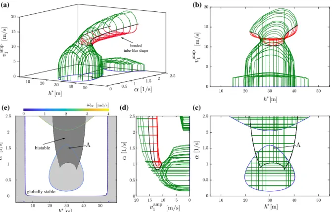
Fig. 10 Three-dimensional wire frame representation of the periodic orbits where the amplitudev1^ampis plotted as a function ofh^∗ andα for parametersβ1 = 0.3 1/s andβ2 = 0 1/s.a three-dimensional isometric view.b–ddifferent projections into 2-dimensional parameter planes. Green and red curves

present stable and unstable periodic orbits, respectively, while black curves visualize their fold bifurcation points.ethe linear stability chart is extended with bistable parameter domain (dark gray area), where different types of solutions coexist. (Color figure online)

Forh^∗ = 30 m, the oscillations of the automated vehicle are depicted in Fig.9as phase-plane plots and as time profiles. Again the cases with and without acceleration saturation are distinguished as solid and dashed curves. Note that the amplitude of the oscillations may be different for different cars. Which vehicle reaches the acceleration saturation limit depends on selected parameters, but the amplitude of oscillations decreases for all vehicles due to the saturation. Furthermore, there exist scenarios, where the acceleration is saturated at both upper and lower boundaries.

In order to get a clear view of the global dynamics, the bifurcation diagram is extended along the control parameterαresulting in a three-dimensional wire frame representation of the periodic orbits shown in Fig.10, where the peak-to-peak amplitudev₁^ampis plotted as a function of parametersh^∗ andα. The three-

dimensional isometric view (Fig.10a) and its different projections (front, top, right) into parameter planes (Fig.10b–d) are presented to help the visualization of the structure.

We generate these figures as follows. First, we per- form similar continuation of the periodic orbits as in Fig.8for numerousαvalues (corresponding to horizontal lines in Fig.10c, d). Second, we fix the parameter h^∗and make similar continuation alongα(vertical lines in Fig.10b, c). Finally, in order to explore the full set of periodic branches, we continue from existing periodic orbits while varying both bifurcation parameters. Note that these steps are necessary to discover global dynamics leading to the bended tube-like shape in Fig.10a, where each cross section along directionh^∗shows an isola for largerαvalues. Stable and unstable periodic orbits are colored with green and red curves, respec-

(10)

(a) (b)

(c) (d)

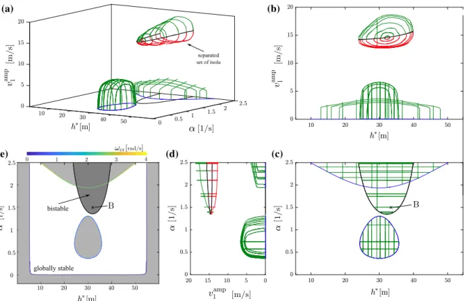
(e)

Fig. 11 Three-dimensional bifurcation diagram of the periodic orbits in case of separated isola, where the amplitudev^amp1 is plotted as a function ofh^∗andαforβ1=0.3 1/s andβ2=0.15 1/s.aThree-dimensional isometric view.b–dDifferent projections into 2-dimensional parameter planes. Green and red curves

present stable and unstable periodic orbits, respectively, while black curves visualize their fold bifurcation points.eThe linear stability chart extended with bistable parameter domain (dark gray area), where different types of solutions coexist. (Color figure online)

(a) (b)

Fig. 12 Phase portrait representation of periodic orbits at a bistable scenario for parameter point A in Fig.10, where an unstable equilibrium (red cross) and an unstable periodic orbit (red curve) coexist with two stable periodic orbits (green curves).

The parameters areh^∗ =32 m,α =1.5 1/s,β1=0.3 1/s and β2=0 1/s. (Color figure online)

tively. Fold bifurcation points, where branches of stable and unstable oscillations meet, are marked by black curves. These are generated by 2-parameter continua-

(a) (b)

Fig. 13 Phase portrait representation of periodic orbits at a bistable scenario for parameter point B in Fig.11, where a stable equilibrium (green cross) and a stable periodic orbit (green curve) are “separated” by an unstable periodic orbit (red curve).

The parameters areh^∗=32 m,α=1.5 1/s,β1=0.3 1/s and β2=0.15 1/s. (Color figure online)

tion in DDE-Biftool, and they bound the bistable area that is highlighted as a dark gray domain in Fig.10e, as an extension of the linear stability diagram.

(11)

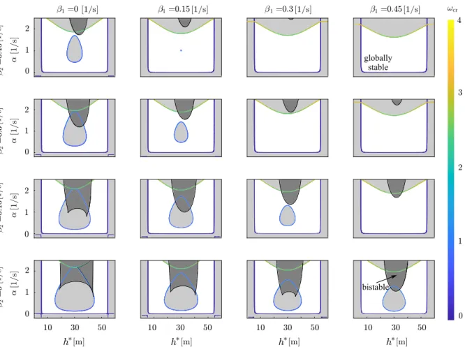
Fig. 14 Stability charts with linearly unstable (light gray) and bistable (dark gray) domains for different values ofβ1andβ2as indicated

In Fig.11a, similar 3D-bifurcation diagram is visu- alized, but for a positiveβ2value (when the automated vehicle can have access for information beyond-line- of-sight). In this case, the bended tube-like shape is separated from the periodic orbits arising from equilibria. In this way, a set of isolas appear that are not connected to periodic branches arising from equilibria (see Fig.11a, b and d).

The appearance of isola results in a bistable solution in two different scenarios: (i) two stable periodic orbits coexist or (ii) a stable equilibrium solution and a periodic orbit coexist. Scenario (i) can be found only above the linearly unstable equilibrium solution, which is already a practically unfavorable regime. In order to illustrate this case, point A is selected in Fig.10c and e and oscillations are plotted for stable (green curves) and unstable (red curve) periodic orbits in the phase plane in Fig.12where the unstable equilibrium is denoted

by red cross. In scenario (ii), the system may approach the equilibrium or the a periodic orbit depending on the initial conditions. This case is illustrated for parameter point B, noted in Fig.11c and e. The corresponding phase portraits are shown in Fig.13a and b where the stable equilibrium is denoted by green cross.

The role of the unstable oscillation is that it “sepa- rates” the basins of attractions of the two stable states (in the infinite dimensional state space). In other words, it determines the threshold for the strength of perturbations, which is necessary to “transfer” the systems from uniform flow to stop-and-go motion. Over-the- threshold perturbations may trigger stop-and-go traffic jams even when the uniform flow is linearly stable.

Again, the bistable region is denoted by a dark gray area in Fig.11e.

The final goal of parameter analysis is to ensure globally stable behavior of the traffic flow, that is, to

(12)

extend the linear stability charts in Fig. 6 with the bistable regions as in Figs.10e and11e. This way, we can represent the influence of all the parameters and the global dynamics. This is summarized in Fig.14, where only parameters within the white globally stable domains are favorable. Similar to linearly unstable droplet, the bistable domain shrinks when increasing β1andβ2. However, notice that theβ2parameter has a stronger effect on the reduction in the unsafe bistable domain.

It should be noted that without utilizing information from beyond-line-of-sight (β2=0), neither the droplet nor the bistability can be eliminated within reasonable control parameters. For this case, we need very large β1to push the bistable domain up to the upper linearly unstable area. On the other hand, utilizing beyond-line- of-sight information (β2 > 0), moderate parameters can be selected. During the design of the control, with the knowledge of the parameter uncertainties, we can select robust control parameters from the globally stable parameter domain (e.g.,α=0.5 1/s,β1=0.3 1/s, β2 = 0.3 1/s). In other words, these results allow us to identify those parameters where heterogeneous connected vehicle system is efficient and still robustly stable. These parameters were used in experimental validation of connected automated vehicle among human- driven vehicles in [12,13].

6 Conclusion

In this paper, heterogeneous connected vehicle systems were investigated, which include human-driven as well as connected automated vehicles. The reaction time delay of human drivers as well as the communication and actuation delays of connected automated vehicles was taken into consideration. Saturations due to the speed limit and limited acceleration capabilities of the vehicles were also incorporated. The arising nonlinear delayed system was studied using analytical and numerical bifurcation analyses. Linear stability analysis was used to identify regions in parameter space, where oscillations arose due to loss of stability of the equilibrium. Robust stability charts were drawn that can be used to ensure linear stability independent of the average headway (that changes as traffic becomes more dense) and the gain used for distance control (which is often chosen according to safety considera- tions). Moreover, with the help of numerical continua-

tion, we determined the bistable regions, where smooth traffic flow coexists with congested states and sufficiently large perturbations may trigger traffic waves.

We demonstrated that utilizing beyond-line-of-sight information (that is obtained via V2V communication), a connected automated vehicle is able to completely eliminate traffic waves at both the linear and nonlinear levels.

Acknowledgements Open access funding provided by Budapest University of Technology and Economics (BME). This work was partially funded by the Hungarian EMMI ÚNKP- 18-3-I New National Excellence Program of the Ministry of Human Capacities and the National Science Foundation (Award No. 1351456). The research reported in this paper was sup- ported by the Higher Education Excellence Program of the Min- istry of Human Capacities in the frame of Artificial intelligence research area of Budapest University of Technology and Eco- nomics (BME FIKP-MI).

Compliance with ethical standards

Conflict of interest The authors declare that they have no conflict of interest.

Open Access This article is distributed under the terms of the Creative Commons Attribution 4.0 International License (http://

creativecommons.org/licenses/by/4.0/), which permits unrestr- icted use, distribution, and reproduction in any medium, provided you give appropriate credit to the original author(s) and the source, provide a link to the Creative Commons license, and indicate if changes were made.

References

1. di Bernardo, M., Salvi, A., Santini, S.: Distributed consensus strategy for platooning of vehicles in the presence of time varying heterogeneous communication delays. IEEE Trans.

Intell. Transp. Syst.16(1), 102–112 (2015)

2. Milanes, V., Shladover, S.E.: Modeling cooperative and autonomous adaptive cruise control dynamic responses using experimental data. Transp. Res. Part C48, 285–300 (2014)

3. Shladover, S.E., Nowakowski, C., Lu, X.-Y., Ferlis, R.:

Cooperative adaptive cruise control definitions and operat- ing concepts. Transp. Res. Rec.2489, 145–152 (2015) 4. Zhou, Y., Ahn, S., Chitturi, M., Noyce, D.A.: Rolling hori-

zon stochastic optimal control strategy for ACC and CACC under uncertainty. Transp. Res. Part C83, 61–76 (2017) 5. Lioris, J., Pedarsani, R., Tascikaraoglu, F.Y., Varaiya, P.:

Platoons of connected vehicles can double throughput in urban roads. Transp. Res. Part C77, 292–305 (2017) 6. Turri, V., Besselink, B., Johansson, K.H.: Cooperative look-

ahead control for fuel-efficient and safe heavy-duty vehicle platooning. IEEE Trans. Control Syst. Technol.25(1), 12–28 (2017)

(13)

7. Zheng, Y., Li, S.E., Li, K., Borrelli, F., Hedrick, J.K.: Dis- tributed model predictive control for heterogeneous vehicle platoons under unidirectional topologies. IEEE Trans. Con- trol Syst. Technol.25(3), 899–910 (2017)

8. Jiang, H., Hu, J., An, S., Wang, M., Park, B.B.: Eco approaching at an isolated signalized intersection under partially connected and automated vehicles environment.

Transp. Res. Part C79(Supplement C), 290–307 (2017) 9. Luo, Y., Xiang, Y., Cao, K., Li, K.: A dynamic automated

lane change maneuver based on vehicle-to-vehicle communication. Transp. Res. Part C62, 87–102 (2016)

10. Ge, J.I., Orosz, G.: Connected cruise control among human- driven vehicles: experiment-based parameter estimation and optimal control design. Transp. Res. Part C95, 445–459 (2018)

11. Stern, R., Cui, S., Delle Monache, M.L., Bhadani, R., Bunting, M., Churchill, M., Hamilton, N., Haulcy, R., Pohlmann, H., Wu, F., Piccoli, B., Seibold, B., Sprinkle, J., Work, D.: Dissipation of stop-and-go waves via control of autonomous vehicles: field experiments. Transp. Res. Part C7(1), 42–57 (2018)

12. Ge, J.I., Avedisov, S.S., He, C.R., Qin, W.B., Sadeghpour, M., Orosz, G.: Experimental validation of connected automated vehicle design among human-driven vehicles. Transp.

Res. Part C91, 335–352 (2018)

13. Avedisov, S.S., Bansal, G., Kiss, A.K., Orosz, G.: Exper- imental verification platform for connected vehicle net- works. In: Proceedings of the 21st International Conference on Intelligent Transportation Systems, pp. 818–823. IEEE (2018)

14. Zhang, L., Orosz, G.: Motif-based design for connected vehicle systems in presence of heterogeneous connectivity structures and time delays. IEEE Trans. Intell. Transp. Syst.

17(6), 1638–1651 (2016)

15. Bachrathy, D., Stépán, G.: Improved prediction of stability lobes with extended multi frequency solution. CIRP Ann.

Manuf. Technol.62, 411–414 (2013)

16. Engelborghs, T.K., Samaey, G.: DDE-Biftool v. 2.00: a Mat- lab package for bifurcation analysis of delay differential equations. Technical Report TW-330, Department of Com- puter Science, K.U. Leuven, Leuven, Belgium (2001) 17. Sieber, J., Engelborghs, K., Luzyanina, T., Samaey,

G., Roose, D.: DDE-Biftool manual—bifurcation analysis of delay differential equations. Tech. rep. (2014).

arXiv:1406.7144

18. Orosz, G., Wilson, R.E., Krauskopf, B.: Global bifurcation investigation of an optimal velocity traffic model with driver reaction time. Phys. Rev. E70, 026207 (2004)

19. Stépán, G.: Retarded Dynamical Systems: Stability and Characteristic Functions. Longman, Harlow (1989) 20. Insperger, T., Stépán, G.: Semi-discretization for Time-

Delay Systems, vol. 178. Springer, New York (2011) 21. Kolmanovskii, V.B., Nosov, V.R.: Stability of Functional

Differential Equations. Academic Press, London (1986) 22. Bachrathy, D., Stépán, G.: Bisection method in higher

dimensions and the efficiency number. Periodica Polytech.

Mech. Eng.56(2), 81–86 (2012)

23. Bachrathy, D.: Robust stability limit of delayed dynamical systems. Periodica Polytech. Mech. Eng.59(2), 74–80 (2015)

Publisher’s Note Springer Nature remains neutral with regard to jurisdictional claims in published maps and institutional affil- iations.