Robust design of connected cruise control among human-driven vehicles
D´avid Hajdu, Jin I. Ge, Tam´as Insperger, and G´abor Orosz
Abstract—This paper presents the robustness analysis for the head-to-tail string stability of connected cruise controllers that utilize motion information of human-driven vehicles ahead. In particular, we consider uncertainties arising from the feedback gains and reaction time delays of the human drivers. We utilize the linear fractional transformation and the M-∆ uncertain interconnection structure to represent the uncertainties in the block-diagonal matrix ∆. The uncertain gains are directly incorporated in the uncertain interconnection structure, while the uncertain time delays are taken into account using the Rekasius substitution that preserves the tightness of the robustness bounds.
This modeling framework scales well for large-size connected vehicle systems. We demonstrate through two case studies how parameters in the connected cruise controller can be selected to ensure robust string stability. Theoretical results are supported by experiments that highlight the advantage of robust control designs.
Index Terms—Connected vehicles, Robustness, Structured sin- gular values.
I. INTRODUCTION
O
VER the past few decades, passenger vehicles are equipped with more and more automation features in order to improve active safety, passenger comfort, and traffic efficiency of the road transportation system. In particular, adaptive cruise control (ACC) was invented to automate the longitudinal dynamics and alleviate human drivers from the constant burden of speed control [1]. While the influence of ACC is yet to be observed in real traffic due to its low penetration rate, theoretical studies have found that automated vehicles may have limited benefits on traffic flow [2], [3].In particular, ACC vehicles may not be able to effectively suppress the speed fluctuations propagating through the ve- hicle string, as each vehicle only responds to its immediate predecessor [4].
In order to overcome such limitations in an automated vehicle platoon, cooperative adaptive cruise control (CACC) was proposed using vehicle-to-vehicle (V2V) communication
D´avid Hajdu is with the Department of Applied Mechanics, Budapest University of Technology and Economics, Budapest, Hungary, e-mail:
hajdu@mm.bme.hu
Jin I. Ge is with the Department of Computing and Mathematical Sci- ences, California Institute of Technology, Pasadena, CA 91125, USA, e-mail:
gejin@umich.edu
Tam´as Insperger is with the Department of Applied Mechanics, Budapest University of Technology and Economics and MTA-BME Lend¨ulet Human Balancing Research Group, Budapest, Hungary, e-mail:
insperger@mm.bme.hu
G´abor Orosz is with the Department of Mechanical Engineering and with the Department of Civil and Environmental Engineering, University of Michigan, Ann Arbor, MI 48109, USA, e-mail: orosz@umich.edu
Manuscript accepted January 28, 2019.
[5], [6], [7], [8]. CACC has been shown to improve fuel econ- omy and traffic efficiency in both theoretical and experimental studies [9], [10], [11], [12]. However, the application of CACC in the early stages of driving automation may be significantly limited by the requirement that all vehicles in a CACC platoon must be automated aside from being equipped with vehicle- to-everything (V2X) communication devices [13], [14]. In particular, as mentioned in [15], “at low market penetrations, ... the probability of consecutive vehicles being equipped is negligible”. Given the relatively low cost of V2X devices compared with ACC and other driving automation systems, it is desirable to exploit the benefits of V2X without being restricted by the penetration rate of automation. Thus, we need to consider a connected automated vehicle design that is able to utilize V2X information sent from human-driven vehicles ahead.
For the longitudinal control of such a connected automated vehicle design, we proposed a class of connected cruise controllers (CCC) that exploit ad-hoc V2X communication with multiple human-driven vehicles ahead [16]. By utilizing motion information from multiple vehicles ahead, connected cruise control is able to gain “phase lead” as it responds to speed fluctuations propagating along the vehicle chain [17].
Several theoretical studies have shown that connected cruise control is able to significantly improve active safety, fuel economy, and traffic efficiency of the connected automated vehicle, especially by providing head-to-tail string stability [18], [19], [20], [21].
Safety, stability and efficiency are important requirements that the automated vehicle must meet even in case of partially known vehicle parameters and external disturbances. Since connected automated vehicle design relies on models, uncer- tainties need to be considered to guarantee robust performance of the connected vehicle system. In order to guarantee robust performance, H∞ framework was often used to synthesize controllers. For example, anH∞-controller for a discrete time system with Markovian jumping parameters was introduced by [22], a centralized controller design using a mixed H2/H∞ method was used in [23], while a decentralized solution without a designated platoon leader was presented in [10].
A distributed H∞-controller was investigated in [24], [25], and a similar approach with a heterogeneous vehicular platoon was studied in [26]. Some other methods were also used in [27], [28], [29], [30], [31], [32] in order to discuss the effects of unmodeled dynamics, stochastic communication delay, measurement noise, and external disturbances.
However, the H∞ approach typically gives conservative results as pointed out in [26]. Consequently, this approach
n. 2. 1. 0.
n+1.
...
h0
h1 l
l 1
2 l
... 0
v2 v1 v0
Fig. 1. A connected vehicle network arising from the V2V-based controller of a connected automated vehicle.
may be feasible for scenarios of limited uncertainty where all vehicles are automated and the connectivity topology is set by the designer. On the other hand, such conservativeness cannot be tolerated when a connected automated vehicle needs to respond to multiple human drivers using ad-hoc communication. There is a need for a systematic method to guarantee robust string stability against human drivers ahead with uncertain reaction time delay and feedback gains. In particular, uncertainties in the time delay must be taken into account without using conservative approximations. Moreover, the control design should allow flexible connectivity topology and scale well as the number of vehicles connected by V2X communication increases. Therefore, in this paper, we adopt structured singular value analysis [33], [34], in order to provide tight bounds for connected cruise controllers to be robustly head-to-tail string stable, despite uncertainties in human car- following behavior. We demonstrate through experimental results how this robust string stability may improve the perfor- mance of a connected automated vehicle among human-driven vehicles.
The paper is structured as follows. Sec. II introduces con- nected vehicle networks including the car-following models of human drivers and the structure of the controller for connected automated vehicles. Sec. III gives the detailed derivation of the uncertain model, introduces the structured singular values, and presents the results for a simple vehicle configuration. Sec. IV extends the results for large connected vehicles networks, and uses a four-vehicle system for demonstration purposes.
This four-vehicle system is implemented in an experiment and the measurement results are discussed in Sec. V. Finally, in Sec. VI we reach the conclusions and provide some future research directions.
II. CONNECTED VEHICLE SYSTEMS
In this section we describe the longitudinal dynamics of a connected vehicle system. We consider a heterogeneous chain of vehicles where all vehicles are equipped with V2V commu- nication devices and some are capable of automated driving, as shown in Fig. 1. When an automated vehicle receives motion information broadcasted from several vehicles ahead, it may choose to use the information in its motion control (see the dashed arrows), and thus, it becomes a connected automated vehicle. Such a V2V-based controller then defines a connected vehicle network consisting of the connected automated vehicle and the preceding vehicles whose motion signals are used by the connected automated vehicle.
Inside this connected vehicle network, we denote the con- nected automated vehicle as vehicle 0, and the preceding vehicles as vehicles1, . . . , n. Note that we assume a connected automated vehicle does not “look beyond” another connected automated vehicle. For example, in Fig. 1, if vehicle2was also a connected automated vehicle, vehicle 0 would not include the V2V signals from vehicles farther ahead than vehicle 2 in its controller. This assumption greatly simplifies the topology of connected vehicle networks and eliminates intersections of links that are typically detrimental for the performance of the system [18], [35].
Time delays naturally arise in connected vehicle systems due to powertrain dynamics, reaction time delays of human drivers, communication delays or packet losses. The different sources of delays and effects on stability have been widely studied in the literature and have also been verified experimen- tally [10], [16], [25], [36], [37], [38], [39]. Stability and control of platooning in the presence of time-varying delays was also investigated in [38], [40], and predictor based designs were introduced in [41], [42] in order to overcome the destabilizing effects of delays.
The longitudinal dynamics of vehicleican be described by h˙i(t) =vi+1(t)−vi(t),
˙
vi(t) =ui(t−ξi), (1) for i= 0, . . . , n, wherehi,vi andui are the headway, speed and acceleration command of vehicle i, and ξi denotes the actuator delay. Since vehicles1, . . . , nonly use motion infor- mation from their immediate predecessor, their acceleration command can be described by
ui(t) =αi Vi hi(t−τˆi)
−vi(t−τˆi) +βi vi+1(t−τˆi)−vi(t−ˆτi)
, (2)
whereτˆi is the reaction time delay of a human driver or the sensor delay of an automated car, while αi and βi are the control gains. Furthermore,Vi(hi)is the range policy function that describes the desired velocity based on headway. Here we consider
Vi(hi) =
0 if hi ≤hst,i, κi(hi−hst,i) if hst,i< hi< hgo,i, vmax if hi ≥hgo,i,
(3)
whereκi=vmax/(hgo,i−hst,i). That is, the desired velocity is zero for small headways (hi≤hst,i) and equal to the speed limit vmax for large headways (hi ≥ hgo,i). Between these,
the desired velocity increases with the headway linearly, with gradient κi. Note that when hst,i = 0 [m], 1/κi is often referred to as the time headway. Many other range policies may be chosen, but the qualitative dynamics remain similar if the above characteristics are kept.
Unlike many cooperative adaptive cruise control algorithms, the preceding vehicles 1, . . . , n in the connected network shown in Fig. 1 are not required to cooperate with the connected automated vehicle. That is, aside from broadcasting their motion information through V2V communication, no automation of these vehicles is required. Consequently, the feedback gains, the range policy and time delay in (2) cannot be tuned for the connected automated vehicle design. However, the connected automated vehicle 0 may fully exploit V2V signals from vehicles 1, . . . , n with no constraint on the connectivity topology.
Here we consider the longitudinal controller for the con- nected automated vehicle in the form of
u0(t) =a1,0 V0 h0(t−σˆ1,0)
−v0(t−σˆ1,0) +
n
X
j=1
bj,0 vj(t−σˆj,0)−v0(t−σˆj,0) , (4) where the control gains aj,0 and bj,0 and communication delay σˆj,0 correspond to the links between vehiclej and the connected automated vehicle0. Note that the delayσˆj,0arises from communication intermittency and possible packet losses.
Here the range policy functionV0(h0)is defined as in (3) with gradient κ0 for hst,0 ≤h0 ≤hgo,0 that can be tuned by the designer together with the feedback gains aj,0 andbj,0.
Note that when n = 1, the connected automated vehicle only uses motion information from its immediate predecessor, and (4) gracefully degrades to the same control structure as human-driven vehicles [43] or automated vehicles without connectivity [4].
We consider the stability of the connected vehicle system (1,2,4) around the uniform traffic flow, where vehicles travel with the same speedvi(t) =v∗and their corresponding head- ways are hi(t) =h∗i such that Vi(h∗i) =v∗ for i= 0, . . . , n.
We define the perturbations about the equilibrium (h∗i, v∗)as
˜hi(t) =hi(t)−h∗, v˜i(t) =vi(t)−v∗. (5) Since we are interested in how the speed perturbations˜viprop- agate through the connected vehicle system, especially how a connected automated vehicle attenuates such perturbations, we linearize (1,2,4) around the equilibrium(h∗i, v∗)and obtain
h˙˜0(t) = ˜v1(t)−v˜0(t),
˙˜
v0(t) =a1,0 κ0˜h0(t−σ1,0)−˜v0(t−σ1,0) +
n
X
j=1
bj,0 ˜vj(t−σj,0)−v˜0(t−σj,0) , h˙˜i(t) = ˜vi+1(t)−v˜i(t),
˙˜
vi(t) =αi κi˜hi(t−τi)−v˜i(t−τi) +βi v˜i+1(t−τi)−˜vi(t−τi)
, i= 1, . . . , n, (6) where the aggregated delays are σ1,0 =ξ0+ ˆσ1,0 and τi = ξi+ ˆτi.
We assume that the connected vehicle system (6) is plant stable, that is, when the input perturbation ˜vn+1(t)≡0, the perturbations ˜hi, ˜vi of the preceding vehicles and ˜h0, ˜v0 of the connected automated vehicle tend to zero regardless of the initial conditions. Then, we focus on how the connected automated vehicle responds to speed fluctuations propagating through the system. When the speed perturbation v˜0 of the connected automated vehicle has smaller amplitude than the inputv˜n, we call the connected automated vehicle design head- to-tail string stable. Note, that while plant stability of vehicles can be guaranteed by their own parameters, head-to-tail string stability relies on the entire connected topology, and therefore it is a more severe requirement.
The notion of string stability between two consecutive vehi- cles was previously used to explain the amplification of speed perturbations along a chain of vehicles without connectivity [44]. However, by considering head-to-tail string stability we allow speed perturbations to be amplified among the uncon- trollable vehicles1, . . . , n, and we focus on how the connected automated vehicle attenuates the perturbations. Being head- to-tail string stable not only enables a connected automated vehicle to enjoy better active safety, energy efficiency, and passenger comfort, it can also help to attenuate traffic waves [18].
We assume zero initial conditions for (6) and obtain V˜0(s) =
n
X
i=1
Ti,0(s) ˜Vi(s), V˜i(s) =Ti+1,i(s) ˜Vi+1(s),
(7)
whereV˜0(s)andV˜i(s)denote the Laplace transform of˜v0(t) and˜vi(t)for i= 1, . . . , n, and the link transfer functions are
T1,0(s) = (a1,0κ0+b1,0s)e−sσ1,0 s2+a1,0(κ0+s)e−sσ1,0+Pn
l=1bl,0se−sσl,0 , Ti,0(s) = bi,0se−sσi,0
s2+a1,0(κ0+s)e−sσ1,0+Pn
l=1bl,0se−sσl,0 , Ti+1,i(s) = (αiκi+βis)e−sτi
s2+ (αiκi+ (αi+βi)s)e−sτi.
(8) Thus, the head-to-tail transfer function of the connected vehi- cle system is
Gn,0(s) = V˜0(s)
V˜n(s) = det T(s)
, (9)
where the transfer function matrix is T(s) =
T1,0(s) −1 0 · · · 0
T2,0(s) T2,1(s) −1 · · · 0
... ... ... . .. ...
Tn−1,0(s) Tn−1,1(s) Tn−1,2(s) · · · −1 Tn,0(s) Tn,1(s) Tn,2(s) · · · Tn,n−1(s)
,
(10) see [18] for the proof. Note that the minors of (10) can be used to track the propagation of perturbations between any two
vehicles in the system, that is, the transfer function between vehicle iand a preceding vehiclej is
Gj,i(s) = V˜i(s)
V˜j(s) = det Tj,i(s)
, (11)
wherej > iand
Tj,i(s) =
Ti+1,i(s) −1 · · · 0
... ... . .. ...
Tj−1,i(s) Tj−1,i+1(s) · · · −1 Tj,i(s) Tj,i+1(s) · · · Tj,j−1(s)
.
(12) The criterion for head-to-tail string stability at the linear level is guaranteed if the perturbations are attenuated for any frequency, that is,
det T(iω)
<1, ∀ω >0, (13) where we substituted s= iω. In order to facilitate robustness analysis we rewrite (13) as
1−det T(iω)
δc6= 0, ∀ω >0, (14) where δc is an arbitrary complex number inside the unit circle in the complex plane, that is, δc ∈ C and |δc| < 1.
Since (13, 14) only require speed fluctuations to be attenuated between the head vehicle and the automated vehicle, the human-driven vehicles in between can be string unstable.
While the human drivers may amplify speed fluctuations, we assume they behave rationally, that is, they are plant stable.
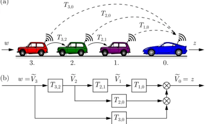
To illustrate the head-to-tail string stability, here we consider a connected automated vehicle using motion information from three vehicles ahead, as shown in Fig. 2(a). The transfer function matrix for this connected vehicle system is
T(s) =
T1,0(s) −1 0 T2,0(s) T2,1(s) −1 T3,0(s) 0 T3,2(s)
, (15) where the elements T1,0(s), T2,0(s), T3,0(s), T2,1(s) and T3,2(s)are given by (8), while (10) results in the head-to-tail transfer function
G3,0(s) = det T(s)
=T3,0(s) +T3,2(s)T2,0(s)+
T3,2(s)T2,1(s)T1,0(s). (16) The flow of information is illustrated on a schematic block diagram in Fig. 2(b).
We consider the case when the preceding vehicles i= 1,2 have the parameters αi = 0.2 [1/s], βi = 0.4 [1/s], κi = 0.6 [1/s],τi= 0.9 [s], and we set the design parameters to a1,0 = 0.4 [1/s], b1,0 = 0.2 [1/s], b2,0 = 0.3 [1/s], b3,0 = 0.3 [1/s], κ0 = 0.6 [1/s] while having the delays σ1,0=σ2,0=σ3,0=σ= 0.6 [s]for the connected automated vehicle. Human driver parameters are experimentally identified by [37], which results string unstable link transfer functions T2,1(iω)andT3,2(iω).
In Fig. 3(a) we plot the head-to-tail transfer function
|G3,0(iω)| of the connected automated vehicle (solid blue curve) and the link transfer function|T3,2(iω)| that describes how vehicle 2 responds to the motion of vehicle 3 (dotted
T3,0
T2,0
T1,0
3. 2. 1. 0.
z w
T2,1
T3,2 (a)
(b)
T1,0 T2,0 T3,0 V~3 V
2
~ V
1
~ V
0
~ T2,1
T3,2 = z
w =
Fig. 2. A four-vehicle configuration: (a) Connected vehicle network with the information flow indicated by the dashed arrows. (b) The corresponding block diagram showing the propagation of speed perturbationsV˜i(s), fori= 3,2,1,0.
t [s]
10 20 30 40
15 25
5
t [s]
10 20 30 40
30 50
10
vi [m/s]hi [m]
[rad/s]
0 1 2 3
Amplification
0 0.2 0.4 0.6 0.8
(a) (b)
)|
|T3,2(
|G3,0( )|
|T2,1( )|
1.0 1.2
0.5
i i i
Fig. 3. (a) Example transfer functions|T3,2(iω)|=|T2,1(iω)|,|G3,0(iω)|
and (b) corresponding simulations withv∗ = 15 [m/s],vamp3 = 5 [m/s], andω= 0.5 [rad/s].
green curve). Here this is equal to |T2,1(iω)| (point-dotted purple curve) as vehicles 2 and 1 have the same parameters.
While the magnitude of the head-to-tail transfer function stays below 1, the link transfer functions of vehicles 2 and 1 reach beyond 1 for low frequencies. This indicates that speed perturbations at low frequency are amplified by vehicles 2 and 1 but eventually are suppressed by the connected automated vehicle 0. This observation is supported by a simulation shown in Fig. 3(b), where the speed inputv3(t) =v∗+v3ampsin(ωt) with v∗ = 15 [m/s], vamp3 = 5 [m/s], ω = 0.5 [rad/s] is plotted as a dashed red curve. The time profiles for vehicles 2 and 1 are plotted by dotted green and point-dotted purple curves, respectively. The color code corresponds to the vehicle colors in Fig. 2(a).
Note that the results shown in Fig. 3 strongly depend on the parameters of the preceding vehicles. The same control parameters used in Fig. 3 may behave poorly with a different set of parametersκi,αi,βiandτi. In the forthcoming sections, we will assume additive perturbation in these parameters denoted byκ˜i,α˜i,β˜i andτ˜i, and apply robust control design to ensure good performance under these parameter changes.
III. ROBUST STRING STABILITY
Since a connected automated vehicle may not know the dynamics of the preceding vehicles 1, . . . , n accurately, the
V2V-based controller should be robust against their param- eter uncertainties aside from the model uncertainties of the connected automated vehicle itself. Based on the theory of robust control, we represent the system uncertainty in the M-∆uncertain interconnection structure, as shown in Fig. 4.
Here,M(s)represents the interconnection transfer function matrix (generalized plant) with scalar input w and scalar output z, while ∆(s) contains bounded perturbations with y and u as the uncertainty input and output. The uncertain interconnection structure can represent parametric and non- parametric uncertainties of the linearized system that are all contained in the matrix∆(s). While in general the structure of
∆(s)might be arbitrary, in this work we restrict ourselves to scalar parametric uncertainties. That is, we limit the structure of the uncertainty matrix to
∆(s) = diag [ρ1(s)δ1, . . . , ρl(s)δl], (17) where |δk| < 1 for k = 1, . . . , l, and l is the number of uncertain parameters. Note, that δk can be real (δkr ∈ R) or complex (δck ∈C), depending on the parameter it represents.
For an introductory course in robust analysis and control, see [34], [45], or for similar studies, see [24], [25], [26].
Let us introduce the weight matrix
R(s) = diag [ρ1(s), . . . , ρl(s)], (18) which scales the uncertaintiesδk. In general the weightsρk(s) depend on s (or later simply on ω). However, we will see that in case of parametric uncertainties they often become simple constants. Therefore, the linear model of the system with uncertainty is given by
y z
=M(s) u
w
, (19)
u=∆(s)y, (20) with the interconnection transfer function matrix being parti- tioned as
M(s) =
M1,1(s) M1,2(s) M2,1(s) M2,2(s)
. (21)
HereM2,2(s)is the nominal transfer function. If∆(s)is zero, then the uncertainty drops out of the equation and only the nominal system remains.
Let w = ˜Vn(s) andz = ˜V0(s) denote the velocity pertur- bations of the vehicles at the head and the tail, respectively.
This yields that the transfer function betweenzandwequals to the head-to-tail transfer function including uncertainties. This transfer function can be expressed using upper linear fractional transformation as
Fu M(s),∆(s)
:= (22)
M2,2(s) +M2,1(s)∆(s) I−M1,1(s)∆(s)−1
M1,2(s)
z y u
w M(s) (s)
Fig. 4. M-∆uncertain interconnection structure.
under the condition that
det I−M1,1(s)∆(s)
6= 0. (23) Observe, that if there is no uncertainty present in the system (∆(s) =0), then upper linear fractional transformation gives thatM2,2(s) =Gn,0(s). We also note that (23) is related to the plant stability boundaries under parametric uncertainty. Since plant stability can be guaranteed by most human drivers and automated vehicle designs, we assume that the connected auto- mated vehicle design remains plant stable for the investigated model uncertainties.
Recall the string stability criterion (14). Similarly, the perturbed head-to-tail transfer function (22) needs to satisfy
1− Fu M(iω),∆(iω)
δc 6= 0, ∀ω >0 (24) for any complex number |δc| < 1. Using the Schur formula (see [46]), we rewrite (23) and (24) for s= iω as
det
I 0 0 1
−
M1,1(iω) M1,2(iω) M2,1(iω) M2,2(iω)
∆(iω) 0 0 δc
! 6= 0. (25) Using the weight matrix R(iω), (25) can be rewritten in the compact form
det I−M(iω) ˆˆ ∆
6= 0, (26)
where
M(iω) =ˆ
M1,1(iω)R(iω) M1,2(iω) M2,1(iω)R(iω) M2,2(iω)
, (27)
∆ˆ = diag [δ1, . . . , δl, δc]. (28) Note, that whileδk,k= 1, . . . , l represent parametric uncer- tainty, δc is required to fulfill robust string stability (robust performance).
A. Robust string stable example
In order to quantify the robustness of the system, we use the structured singular value analysis introduced in [33]. We
i+1.
(a)
(b)
i.
1s 1
s
~
~
~
e-s s
, , ,
y1 u1
y2 u2 y3 u3
y4 u4 w =V~i+1 ~
z =V~i
Fig. 5. (a) Predecessor-follower model; (b) Block diagram of the uncertain transfer function.
define the µ-value of M(iω)ˆ as the inverse of the smallest
¯
σ( ˆ∆) when (26) fails at frequencyω, i.e., µ(ω) =
min
∆ˆ
¯σ( ˆ∆) : det I−M(iω) ˆˆ ∆
= 0 −1
, (29) where σ( ˆ¯ ∆) denotes the largest singular value of ∆. Asˆ µ(ω) increases, a smaller perturbation value in ∆ˆ may lead to a singular I−M(iω) ˆˆ ∆
and results in string instability.
When singularity holds for arbitrarily small perturbations, then µ(ω) → ∞ and robustness cannot be guaranteed, however, if det I−M(iω) ˆˆ ∆
6= 0 for any perturbation ∆, thenˆ µ(ω) = 0. Therefore, the condition for robust string stability against bounded parameter variation is
µ(ω)<1, ∀ω >0, (30) otherwise there exists a perturbation matrix ∆,ˆ σ( ˆ¯ ∆) < 1 such that det I−M(iω) ˆˆ ∆
= 0.
The definition ofµaccording to (29) does not yield directly any tractable way to compute it, since the optimization prob- lem is not convex in general, therefore multiple local extrema might exist [47]. Instead, we are interested in computing upper (µ(ω)≤µ(ω)) and/or lower bounds (µ(ω)≤µ(ω)), for which several alternative formulations have been developed, see [33], [47], [48], [49]. In this paper, we use the mussv function in MATLAB µ-Analysis and Synthesis Toolbox [50], which implements these algorithms, and we only focus on the results, not on the numerical issues.
As an illustration of the robust string stability, we consider vehicle i that only uses information from one vehicle ahead;
see Fig. 5(a). In this case the input of the nominal system is
˜
vi+1(t) while the output is v˜i(t). The nominal link transfer function is given by
Ti+1,i(s) = (ακ+βs)e−sτ
s2+ (ακ+ (α+β)s)e−sτ, (31) where, for the sake of brevity, we dropped the subscripts of the parameters κ,α,β, andτ; cf. (8).
While the additive uncertainties α,˜ β, and˜ κ˜ result in additive uncertainty terms, an additive delay uncertainty˜τwill result in a multiplicative exponential term e−s˜τ in (31), that is,
Ti+1,i(s) + ˜Ti+1,i(s) =
(κ+ ˜κ)(α+ ˜α) + (β+ ˜β)s
e−s(τ+˜τ) s2+ (κ+ ˜κ)(α+ ˜α) + (α+ ˜α+β+ ˜β)s
e−s(τ+˜τ), (32)
whereT˜i+1,i(s) represents the uncertainty while the nominal part Ti+1,i(s) is given by (31). In order to clearly separate the model of the single vehicle from the connected vehicle structure, we introduce the notationm-δ and use lower case letters for the single car scenario. In case of multiple vehicles, M(s)and∆(s) can be built up systematically from the link transfer functions Tj,i(s), matrices m(s) and uncertainties δ(s)of individual vehicles (see Sec. IV).
To formulate the uncertainties in a way that can be repre- sented by them-δinterconnection structure (19-20), and make the robust analysis feasible, we use the Rekasius substitution
e−s˜τ = 1−sϑ(s)˜
1 +sϑ(s)˜ , (33) where we restrict ourselves tos= iω and therefore we have
ϑ(iω) =˜ 1 ωtanωτ˜
2 , (34)
see [51]. This substitution is exact in the region 0 ≤ ω <
π/˜τ, since it covers the same domain on the complex plane as e−iω˜τ.
By taking into account the uncertain parameters (and the Rekasius substitution), the block diagram in Fig. 5(b) can be drawn. This illustrates how uncertainties affect the system and allows us to construct them-δ uncertain interconnection structure by solving a number of algebraic equations. In par- ticular, we define the interconnection transfer function matrix m(s) for a single vehicle by (35-36), where the matrix of uncertainties read
δ(s) = diagh
˜
κ,α,˜ β,˜ ϑ(s)˜ i
, (37)
cf. (17). Therefore using (22), the perturbed link transfer function can be written as
Fu m(s),δ(s)
=Ti+1,i(s) + ˜Ti+1,i(s) (38)
= m2,2(s)
| {z } Ti+1,i(s)
+m2,1(s)δ(s) I−m1,1(s)δ(s)−1
m1,2(s)
| {z }
T˜i+1,i(s)
=
(κ+ ˜κ)(α+ ˜α) + (β+ ˜β)s
e−sτ1−sϑ(s)˜ 1 +sϑ(s)˜ s2+ (κ+ ˜κ)(α+ ˜α) + (α+ ˜α+β+ ˜β)s
e−sτ1−sϑ(s)˜ 1 +sϑ(s)˜ .
The only difference compared to (32) is the Rekasius sub- stitution, which is still exact for s = iω. Note that there exist other ways to approximate the uncertainty in the time- delay, for instance by replacing e−s˜τ with a complex term
m(s) = 1 D(s)
−αe−sτ −e−sτ −e−sτ −2 s+αe−sτ
s2+βse−sτ −(κ+s)e−sτ −(κ+s)e−sτ 2(κ+s) κs−βse−sτ
−αse−sτ −se−sτ −se−sτ 2s s2+αse−sτ
αs3e−sτ s3e−sτ s3e−sτ −s3+s κα+s(α+β)
e−sτ (καs2+βs3)e−sτ
αse−sτ se−sτ se−sτ −2s (κα+βs)e−sτ
,
(35) D(s) =s2+ κα+s(α+β)
e−sτ, (36)
g(s) directly, see [52]. However, this typically leads to a conservative solution.
In order to utilize the robust calculation andµ-analysis, we introduce the weight matrix
r(s) = diag [ρ1, ρ2, ρ3, ρ4(s)], (39) where
˜
κ=ρ1δ1r, α˜=ρ2δ2r, β˜=ρ3δ3r, ϑ(s) =˜ ρ4(s)δr4, (40) cf. (18). Thus, the rescaled matrix (28) reads
δˆ= diag [δr1, δr2, δr3, δr4, δc], (41) where upper index indicates whether the uncertainty is real (δkr ∈R) or complex (δkc ∈C), and
ˆ m(iω) =
m1,1(iω)r(iω) m1,2(iω) m2,1(iω)r(iω) m2,2(iω)
, (42)
cf. (27) and (28). The list of the uncertain parameters and their representations are given in Table I. Then with the use of the MATLAB commandmussv[50], the structured singular value of m(iω)ˆ can be calculated for different values ofω.
The parameter κ may be increased/decreased depending on the driver/passenger preferences and the value of τ is influenced by the powertrain and the automated driving system (or the human driver reaction time). Thus, we assume nonzero parameter uncertaintiesκ˜andτ, set˜ α˜ = 0,β˜= 0, and plot the robust string stable regions in the (β, α)-plane. In particular, we quantifyκ˜andτ˜using nominal values with variations. For example,10%inκindicates that the parameter has maximum 10% uncertainty in its nominal value (ρ1 = 0.1κ in (39)).
For simplicity, we assume the same relative uncertainty for κ andτ. In order to speed up the calculations, the bisection algorithm developed in [53] is utilized, and only the boundary is searched.
For parameter values κ = 0.6 [1/s], τ = 0.7 [s], the nominal (black) and robust (gray) string stability boundaries are shown in Fig. 6(a). In this case string stable domain exists when τ < 1/(2κ) ≈ 0.833 [s]. As the uncertainty in κ and τ increases, the robust string stable area shrinks. Note that when uncertainty goes above 8%, the robust stable domain completely disappears.
We pick the point A (α = 0.1 [1/s], β = 0.65 [1/s]) in Fig. 6(a), and plot the corresponding µ(ω) and nominal
|Ti+1,i(iω)| curves in Fig. 6(b-c). The absolute value of the
TABLE I
UNCERTAINTIES IN THE PREDECESSOR-FOLLOWER VEHICLE MODEL. Parameter/
Performance Uncertainty and representation Weight Type Gradientκ κ+ ˜κ=κ+ρ1δr1 ρ1 δr1∈R
Gainα α+ ˜α=α+ρ2δ2r ρ2 δr2∈R Gainβ β+ ˜β=β+ρ3δr3 ρ3 δr3∈R Time delay
τ e−s τ+˜τ
= e−sτ1−sρ1+sρ4(s)δr4
4(s)δr4 ρ4(s) δr4∈R Robust
performance 1− Fu m(iω),δ(iω)
δc6= 0 1 δc∈C
[1/s]
[1/s]
0 0.2 0.4 0.6
0.4 0.5 0.6 0.7 0.8 0.3
0.5 1.0 1.5 2.0 2.5
0 3.0
( )
0 0.2 0.4 0.6 0.8 1.0 1.2
[rad/s]
4 4 0.
2 0 0
6 6
8 8
A A string unstable (a)
(b)
string stable
|Ti+1,i( )|
Upper bound, Lower bound,
i
4 6 8
4
0.4 0.6 0.8 1.0
[rad/s]
0.975 1.00 1.025 1.050
0.950
( )
0 2 (c)
( ) ( )
Fig. 6. (a) Robust stability charts in the (β,α)-plane forκ = 0.6 [1/s], τ= 0.7 [s]with uncertainties0,2,4,6,8%, where black curve indicates the nominal string stability boundary and gray curves indicate the robust string stability boundaries. (b) The nominal transfer function|Ti+1,i(iω)|(black) and µ(ω) curves (gray) for point A (α= 0.1 [1/s],β = 0.65 [1/s]). (c) Zoom in of the critical region, whereµ(ω)>1.
link transfer function is shown by black curve, while the gray curves correspond to the µ(ω)curves for different uncertain- ties. Recall that the realµ-values cannot be determined exactly, so rather upper bounds (µ- solid gray) and lower bounds (µ- dashed gray) are computed. Details in the critical region can be seen in Fig. 6(c), where only a slight difference between the upper and lower bounds can be observed. This results very small conservativeness, and therefore for a safer approximation we assume that µ(ω)≈µ(ω). If µ(ω)remains below 1, then robustness is guaranteed for that perturbation level. Otherwise, the system can lose string stability around the frequency where µ(ω)is above 1. For example, theα,βcombination at point A is robust against 4% uncertainty, and leads to string unstable behavior at 6%.
IV. ROBUST STRING STABLE DESIGN FOR CONNECTED AUTOMATED VEHICLES
In this section, we first introduce a systematic method to extend the robust head-to-tail string stability analysis to gen- eral connected vehicle systems. This yields a linear fractional transformation model, which can be formulated for arbitrary connected vehicle networks with various topology and un- certainty. Then, we demonstrate the method in a connected automated vehicle design where motion information from three vehicles ahead is used.
A. Scaling up the generalized plant matrix
Recall that for the robustness analysis in Sec. III-A, we deduced the interconnection transfer function matrix m(s) graphically using the block diagram in Fig. 5(b). However,
as the number of vehicles in a connected vehicle system in- creases, it is desirable to obtain such matrices algebraically in a systematic manner. Specifically, we treat each vehicle in the connected vehicle system as a subsystem whose uncertainty is described by an m-δ structure as in Sec. III-A. Then we exploit the topology of the connected vehicle system and assemble theM-∆ structure. Note that this formalism allows us to incorporate the uncertainty for an arbitrary number of human drivers, making this method scaleable for large connected vehicle systems.
Again we consider a connected automated vehicle using motion information from n human-driven vehicles ahead, as shown in Fig. 1. Consider the set D of vehicles with uncertainties (not necessarily all of the vehicles in the system are uncertain), where D ⊆ {1, . . . , n}. Based on (19-20), the uncertainty model for vehicle i ∈ D with respect to vehicle i+ 1 is
yi=m(i+1,i)1,1 (s)ui+m(i+1,i)1,2 (s)wi,
zi=m(i+1,i)2,1 (s)ui+m(i+1,i)2,2 (s)wi, (43) where superscript(i+ 1, i)denotes the uncertain link between vehicles i+ 1 and i, see Fig. 7. Note that m(i+1,i)2,2 (s) = Ti+1,i(s), as in Sec. III-A.
Now we can exploit the cascading topology of the system, as vehicles only respond to perturbations from their immediate predecessor, i.e., the input wi of vehicle i is the outputzi+1 of vehicle i+ 1. Therefore, we define w= ˜Vn,z = ˜V0, and expand the model (43) by including uncertainties up from all preceding vehicle p∈ D ∩ {i+ 1, . . . , n}, that is,
yi=m(i+1,i)1,1 (s)ui+m(i+1,i)1,2 (s)Gn,i+1(s)w
+
n
X
p=i+1
m(i+1,i)1,2 (s)m(p+1,p)2,1 (s)Gp,i+1(s)up, (44) where summation only includes the uncertain vehicles,Gj,i(s) is defined in (11) and Gi,i(s) = 1.
This way, we construct the uncertainM-∆interconnection structure as
... yi
... z
=
... ...
· · · [M1,1(s)]i,j · · · [M1,2(s)]i
... ...
· · · [M2,1(s)]j · · · M2,2(s)
| {z }
M(s)
... uj
... w
,
(45) where the elements in M(s)can be obtained systematically:
[M1,1(s)]i,j=
m(i+1,i)1,2 (s)m(j+1,j)2,1 (s)Gj,i+1(s), ifj > i , m(i+1,i)1,1 (s), ifj=i ,
0, ifj < i ,
(46) [M1,2(s)]i=m(i+1,i)1,2 (s)Gn,i+1(s), (47) [M2,1(s)]j=m(j+1,j)2,1 (s)Gj,0(s), (48)
M2,2(s) =Gn,0(s), (49)
for i, j∈ D.
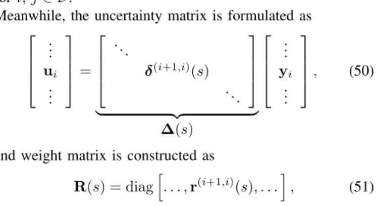
Meanwhile, the uncertainty matrix is formulated as
... ui
...
=
. ..
δ(i+1,i)(s) . ..
| {z }
∆(s)
... yi
...
, (50)
and weight matrix is constructed as R(s) = diagh
. . . ,r(i+1,i)(s), . . .i
, (51)
where δ(i+1,i)(s) and r(i+1,i)(s) are the uncertainty matrix and weight matrix corresponding to vehicle i (cf. (37) and (39)). Finally, robustness is guaranteed if
det I−M(iω) ˆˆ ∆
6= 0, (52)
where
M(iω) =ˆ
M1,1(iω)R(iω) M1,2(iω) M2,1(iω)R(iω) M2,2(iω)
, (53)
∆ˆ = diag [δr1, . . . , δlr, δc]. (54) B. Robust string stability in a four-vehicle system
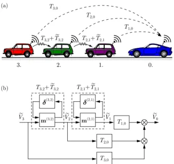
In order to demonstrate the applicability of the algorithm, we present a case study for a connected vehicle system consisting of a connected automated vehicle and three human- driven cars with uncertainty, i.e., n= 3 in (6). The sketch of the system is displayed in Fig. 8(a) while the block diagram with uncertainties is presented in Fig. 8(b), cf. Fig. 2(b).
While the nominal transfer function matrix is given in (15), we assume each parameter in vehicles 2 and 1 has uncertainty and compute the robust string stable regions in the(b2,0, b3,0)- plane for different values ofa1,0 andb1,0.
The uncertain interconnection structure is given as M(s) =
m(2,1)1,1 m(2,1)1,2 m(3,2)2,1 m(2,1)12 T3,2
0 m(3,2)1,1 m(3,2)1,2
m(2,1)2,1 T1,0 m(3,2)2,1 (T2,0+T1,0T2,1) G3,0
, (55)
(j+1,j)
m(j+1,j) uj
Tj+1,j+T~j+1,j
wj =V~j+1
(a)
n j+1 j i+1 i 0
(b)
yj
w =Vn
~ z
j =Vj
~
(i+1,i)
m(i+1,i) ui
Ti+1,i+T~i+1,i
wi =V~i+1
yi
zi =Vi
~ z =V
0
~
Tj+1,j+T~j+1,j T
i+1,i+T~i+1,i
Fig. 7. (a) Chain of connected vehicles with uncertain dynamics. (b) Corresponding block diagram.
T3,0
T2,0
T1,0
3. 2. 1. 0.
T3,2+T~3,2 T
2,1+T~2,1 (a)
(b)
(3,2)
m(3,2) T3,2+T~3,2
(2,1)
m(2,1) T2,1+T~2,1
T1,0
T2,0
T3,0
V~3 V
2
~ V
1
~ V
0
~
Fig. 8. Four-vehicle configuration with uncertainties: (a) Connectivity topol- ogy; (b) Block diagram.
where the dependence on sis not spelled out for conciseness, while the weight matrix reads
R(s) =
r(2,1)(s) 0 0 r(3,2)(s)
. (56)
The robust performance is given by (52-54), where l = 8 corresponds to the 4 + 4 independent parameters of vehicles 1 and 2.
The computation of µ-values are performed by the MAT- LAB toolbox using the mussv function. The results are presented in Fig. 9 and Fig. 10, where we assumed that each parameter of each vehicle is perturbed by the same percentage of their nominal value, i.e., αi, βi, κi and τi have identical relative uncertainties. The nominal human driver parameters are κi = 0.6 [1/s], αi = 0.2 [1/s], βi = 0.4 [1/s] and τi = 0.9 [s] (same for both vehicles for simplicity), while the fixed parameters of the connected automated vehicle are κ0 = 0.6 [1/s]andσ= 0.6 [s]. In this configuration, human- driven vehicles are string unstable, but head-to-tail string stability can be guaranteed by appropriate selection of the gains of the connected automated vehicle. Fig 9. shows how the uncertain parameters (eight in total) affect the robust stable domain of control parameters (a1,0, b1,0, b2,0, b3,0). While the nominal system (black curve) provides a relatively large string stable domain, uncertainty significantly reduces it (gray curves) and having uncertainty greater than 30% eliminates the robust boundaries in most of the cases.
In order to further illustrate the effects of uncertainty, we choose three different control gain pairs in Fig. 10(a) and plot the corresponding µ(ω) curves in Fig. 10(b-d) for different uncertainty levels. Point A (gray) is inside the 20% robustness region and corresponds to b2,0 = 0.3 [1/s], b3,0 = 0.3 [1/s], point B (light red) is inside the 10% robustness region and denotes b2,0 = 0.6 [1/s], b3,0 = 0.0 [1/s], while point C (brown) is outside the 10% robust region, but still inside the
3020 20
10 0
b3,0 [1/s]
1.0 0.5 0
-0.5 0.5 1.0
b2,0 [1/s]
b1,0 = 0.4 [1/s]
-0.5 0 1.5
b3,0 [1/s]
1.0 0.5
0
b1,0 = 0.2 [1/s]
-0.5
b3,0 [1/s]
1.0 0.5
0
b1,0 = 0.1 [1/s]
-0.5
a1,0 = 0.1 [1/s] a1,0 = 0.2 [1/s] a1,0 = 0.4 [1/s]
string stable
2.0 -0.5 0.5 1.0
b2,0 [1/s]
0 1.5 2.0 -0.5 0.5 1.0
b2,0 [1/s]
0 1.5 2.0
string unstable
0 10 3020
0 0 10 10 20 20 20 30 30
0 0 10 10 20 20 20
0 0 10 10 20 20 20 30 30
0 0 10 10 20 20 20 30 30
0 100 10 20 20 20
0 0 10 10 20 20 20
0 0 10 10 20 20 20
0 100 10 20 20 20
Fig. 9. Robust stability charts in the(b2,0, b3,0)-plane for different values ofa1,0andb1,0. The nominal human driver parameters areκi= 0.6 [1/s], αi = 0.2 [1/s],βi = 0.4 [1/s]and τi = 0.9 [s] fori = 1,2, and the connected automated vehicle hasκ0 = 0.6 [1/s]andσ = 0.6 [s]. Robust string stable boundaries are indicated by gray curves in case of0,10,20,30%
uncertainty.
string stable domain and its parameters are b2,0 = 0.2 [1/s], b3,0 = 0.1 [1/s]. Colored thick curves indicate the value of
|G3,0(iω)|, while colored thin curves indicate µ(ω) at 10%
and20%uncertainty levels. In each case the continuous curve is the upper boundµ, while dashed curve is the lower bound µ. The color code used in panel (a) matches the colors on panels (b-d). Similarly to the example shown in Sec. III-A, the shape ofµ-plots are similar to the absolute values of the transfer functions. Where theµ(ω)goes above 1, the system loses string stability around that frequency. If µ(ω) remains below 1, then robustness is guaranteed for the corresponding perturbation level.
V. EXPERIMENTAL VALIDATION OF ROBUST STRING-STABLE DESIGN
In this section we experimentally evaluate the performance of connected cruise control designs with different levels of robustness. We demonstrate that robust string stable design is able to ensure less harsh maneuvers for a connected automated vehicle operating among human-driven vehicles.
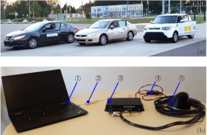
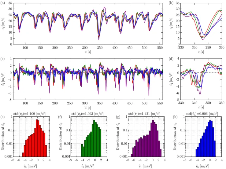
We consider the scenario shown in Fig. 8(a), where one connected automated vehicle drives behind three human- driven vehicles. The connected automated vehicle and two human-driven vehicles used in the experiments are shown in Fig. 11(a). The speed and position data of each vehicle are recorded and transmitted with 10 Hz update rate through dedicated short range communication (DSRC) using V2V devices shown in Fig. 11(b) [54]. We note that while all vehicles are equipped with V2V communication devices, only one vehicle (right) is automated using the connected cruise controller (4). Further details about the setup and experimental


![Fig. 6. (a) Robust stability charts in the (β,α)-plane for κ = 0.6 [1/s], τ = 0.7 [s] with uncertainties 0,2,4,6,8%, where black curve indicates the nominal string stability boundary and gray curves indicate the robust string stability boundaries](https://thumb-eu.123doks.com/thumbv2/9dokorg/1079851.72804/7.918.80.447.958.1111/stability-uncertainties-indicates-stability-boundary-indicate-stability-boundaries.webp)