Research Article
Optimal Control of Overtaking Maneuver for Intelligent Vehicles
Balázs Németh ,
1Péter Gáspár,
1and Tamás Heged4s
21Systems and Control Laboratory, Institute for Computer Science and Control, Hungarian Academy of Sciences, Kende Utca 13-17, H-1111 Budapest, Hungary
2Department of Control for Transportation and Vehicle Systems, Budapest University of Technology and Economics, Budapest, Hungary
Correspondence should be addressed to Bal´azs N´emeth; balazs.nemeth@sztaki.mta.hu
Received 4 June 2018; Revised 28 September 2018; Accepted 10 December 2018; Published 31 December 2018
Academic Editor: Aboelmaged Noureldin
Copyright © 2018 Bal´azs N´emeth et al. This is an open access article distributed under the Creative Commons Attribution License, which permits unrestricted use, distribution, and reproduction in any medium, provided the original work is properly cited.
In the paper a hierarchical overtaking strategy, which is a driver assistance function or rather an autonomous function in electric/autonomous vehicles, is proposed. The solution uses speed and acceleration signals from the surrounding vehicles. These signals are processed with clustering methods in order to achieve probability density functions and predict their expected motion.
The strategy includes several additional layers, such as decision making concerning the maneuver, the computation of the required trajectory, and the tracking control of the vehicle. Trajectory generation is formed as an optimization task, which is able to include the prediction model of the surrounding vehicles in the constraints. A robust Linear Parameter Varying (LPV) control design method is proposed to guarantee the tracking of the computed reference. The proposed strategy is able to guarantee the safe motion of the vehicles and handle the interactions with the other traffic participants.
1. Introduction and Motivation
Overtaking and lane changing maneuvers are critical on roads due to various types of human errors. The necessary distance required by the maneuver must be estimated accu- rately and the vehicle should return to the lane as fast as possible and the maneuver must be safe regarding the other participants in the traffic.
The appropriate handling of overtaking maneuvers is also difficult for several reasons:
(i) The motion of the vehicle ahead must be monitored and predicted
(ii) The motions of vehicles in the environment, espe- cially vehicles coming from the opposite lane and traveling in the return lane, must be monitored and predicted
(iii) The overtaking maneuver must be designed
(iv) Before the maneuver the decision concerning the necessary overtaking must be made
(v) Several factors, such as lateral/longitudinal accel- eration and jerks in relation to comfort, must be considered
(vi) steering, braking, and driving must be coordinated Several different control approaches in the field of over- taking maneuvers of vehicles have been developed. An optimal control design of the overtaking trajectory using polynomial equations to minimize the lateral jerk was pro- posed by [1]. The model predictive control (MPC) method for path planning together with collision avoidance with the application of overtaking was found in [2]. In [3] it has been shown that the nonconvex optimal control problem of the vehicle positioning can be transformed to a convex quadratic program, which can be solved efficiently. A stochastic model predictive control, in which the velocities of the surrounding vehicles are considered, is designed [4]. A mixed integer programming method, which uses a low number of variables, was presented by [5]. Another solution to reduce the numer- ical difficulties was to use linguistic variables. For example, a two-level fuzzy logic control was proposed by [6] and the application of the Q-learning method was demonstrated
Volume 2018, Article ID 2195760, 11 pages https://doi.org/10.1155/2018/2195760
by [7]. The fuzzy logic with the visual system, differential GPS, and inertial measurements was integrated by [8]. Real- time measurement from the overtaken vehicle to generate the vehicle trajectory was used in [9]. A nonlinear adaptive controller design using third-order reference trajectory for overtaking scenarios was proposed by [10].
The prediction of vehicle motions is strongly linked to the overtaking in the field of autonomous vehicles; see, e.g., [11]. With the precise estimation of the environment with vehicles, pedestrians, and cyclists the safe operations of the autonomous systems can be significantly enhanced.
Several methods have also been designed to predict the motion of human-driven vehicles; see, e.g., [12]. Probabilistic approaches based on the dynamic Bayesian network and Markov chain models were found in [13, 14]. A method which used the past similarities in vehicle motion between the current vehicle and predefined number of test vehicles was proposed by [15]. The factor of driver aggression and the motion of vehicles in unorganized traffic were consid- ered in the motion planning of an overtaking maneuver in [16].
In this paper an overtaking strategy of our own vehicle is developed. In the following our vehicle will be referred to as ego vehicle. The overtaking strategy is formed in a hierarchical structure with different layers. The core of the autonomous strategy is the motion prediction of the preced- ing vehicle and surrounding vehicles (e.g., in the opposite lane). Speed and acceleration signals are used to generate probability density functions, which are built in a con- strained optimization structure of the trajectory generation.
The result of the calculation is a clothoid trajectory, which enhances smooth driving and traveling comfort. Moreover, the paper proposes a strategy, with which further vehicle motions can be considered, e.g., following and overtaking the preceding vehicles. The tracking of the designed trajectory is based on the robust LPV vehicle control, which has the important role in guaranteeing safety in all scenarios, such as overtaking, lane changing, and following the preceding vehicle.
1.1. Architecture of the Robust Overtaking Control Strategy.
The overtaking control has been composed of a hierarchical architecture with three different layers, as found in Figure 1.
It contains the layer of the surrounding vehicle motion estimation, the trajectory optimization with an overtaking decision logic, and the vehicle control, which generates the steering angle. The advantage of the hierarchical design is the variation in the design method of the layers. The different tasks of the layers require different approaches;
e.g., the estimation is based on clustering and probability- based methods, and the trajectory design is based on a constrained optimization, while the vehicle control should guarantee robustness. Therefore, it is sufficient to define the interfaces and the layers can be designed independently. In the architecture the interfaces of the layers are the following:
(a) The inputs of the surrounding vehicle estimation block are the longitudinal velocity and the acceleration signals of the ego and the surrounding vehicles, while the outputs are the lateral constraints in the vehicle motion𝑌𝑚𝑖𝑛, 𝑌𝑚𝑎𝑥
Estimation of surrounding vehicle motion
Trajectory optimization and decision strategy
Robust vehicle control for trajectory tracking ego vehicle surrounding vehicles
yref ref x
x
ax x
ax
Ymin Ymax
Figure 1: Architecture of the control system.
(b) Based on the constraints the actual reference signals 𝑦𝑟𝑒𝑓, 𝜓𝑟𝑒𝑓are computed together with the desired longitudinal velocityV𝑥
(c) Finally, the robust vehicle control computes the actual steering angle𝛿
In the rest of the paper the layers of the automated overtaking strategy are presented. The estimation of the surrounding, especially the preceding vehicle motion, which includes the processing of vehicle data and the prediction of its position, is presented in Section 2. The trajectory design is formed in a constrained optimization problem, which is based on a clothoid path of the vehicle; see Section 3. It also shows the decision logic of the overtaking and lane changing maneuvers. The robust vehicle control based on the generated reference signals is presented in Section 4.
The operation of the control system is illustrated through the CarSim simulation environment in Section 5. Finally, Section 6 summarizes the contributions of the paper.
2. Estimation of the Motion of Surrounding Vehicles
Safe overtaking and lane changing maneuvers require infor- mation about the motion of the preceding vehicle. In this paper its motion is estimated using the current longitudinal velocityV𝑥and acceleration𝑎𝑥signals. It is assumed that the motion of the preceding vehicle in the future will be similar to what it has been so far. Moreover, it is also assumed that the required signalsV𝑥and𝑎𝑥are available for the ego vehicles.
The proposed estimation has two main steps. First, the preceding vehicle signals are processed through a clustering procedure and the probability density function is generated.
Second, the future position of the vehicle is predicted based on the calculated density functions.
2.1. Processing of Preceding Vehicle Signals. The preceding vehicle is considered to be driven by a human, whose velocity
−10 −5 0 5 10 15
−15
?P(km/h)
−3
−2.5
−2
−1.5
−1
−0.5 0 0.5 1 1.5 2
;R(m/M2)
Figure 2: Data on preceding vehicle.
selection is determined by a reference velocity V𝑥,𝑟𝑒𝑓. The value ofV𝑥,𝑟𝑒𝑓can depend on several factors, e.g., the speed limitation, the quality of the road surface, the curvature and the number of lanes on the road, and the traffic situation.
In the method the velocity of the human-driven vehicle is compared to the reference velocity, and the difference is computed as𝑒V = V𝑥 −V𝑥,𝑟𝑒𝑓. If several measurements are available from a longer time period, the required signals of the preceding vehicle can be estimated. As an example the relationship between the speed differences 𝑒V and the longitudinal acceleration 𝑎𝑥 is illustrated in Figure 2. In this simplified illustrative scenarioV𝑥,𝑟𝑒𝑓is considered as the speed limit on the course of the vehicle. It is shown that most of the data are around𝑒V = 0,𝑎𝑥 = 0, which means that the vehicle is generally cruising close toV𝑥,𝑟𝑒𝑓. However, the signals have a variance; e.g., if the velocity changes the vehicle is accelerated to reach the speed limit again, which leads to 𝑒V< 0and𝑎𝑥> 0. The purpose of the analysis is to derive the probabilities of the different driving motions of the preceding vehicle.
The generation of probability density functions requires the clustering of data. In this vehicle dynamic examination clustering means that the collected data are ordered in groups, depending on their locations in the plane𝑒V, 𝑎𝑥. Numerous algorithms for this problem have been developed in recent decades; see, e.g., partitioning methods [17], hierarchical algorithms [18], and density based methods [19]. In this paper a fast and efficient improved k-means method is used as presented and analyzed in [20].
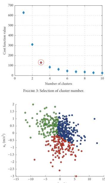
The purpose of the algorithm is to minimize the Euclidean distance between the objects and the centre of the selected cluster, such as
𝐽𝑐𝑙=∑𝐾
𝑖=1
∑𝑁
𝑗=1𝑥𝑗− 𝑐𝑖 (1) where 𝐾 represents the number of clusters, 𝑥𝑗 contains [𝑒V, 𝑎𝑥]object data,𝑁is the number of the objects, and𝑐𝑖∈ 𝐶𝑖
0 100 200 300 400 500 600 700
Cost function value
2 4 6 8 10
0
Number of clusters Figure 3: Selection of cluster number.
−3
−2.5
−2
−1.5
−1
−0.5 0 0.5 1 1.5 2
;R(m/M2)
−10 −5 0 5 10 15
−15
?P(km/h)
Figure 4: Clustered data on preceding vehicle.
is the centre of the cluster𝐶𝑖. The candidate clusters must be nonempty and nonoverlapping.
In the estimation process the number of the clusters significantly influences the results. Several methods have been developed for the determination of the cluster number;
see, e.g., [21]. Below the elbow method is applied. In this case it is necessary to find the cluster number with which the value of the cost function𝐽𝑐𝑙 drops significantly. In our case the elbow method proposes𝐾 = 3clusters; see Figure 3. Result of the clustering is shown in Figure 4, where the clusters are marked with different colours.
Results of the clustering show that the𝑒V,𝑎𝑥 data have variance inside the clusters. Thus, in what follows probability density functions are fitted to the data of each cluster. The function requires a two-dimensional Gaussian form:
𝑓𝑖(𝑥) = 1
(2𝜋)𝑛/2∑𝑖0.5𝑒−0.5(𝑥−𝜇𝑖)𝑇∑𝑖(𝑥−𝜇𝑖), (2)
−15 −10
−5 0 5 10 15
−4
−2 0 2 40 0.05 0.1 0.15 0.2 0.25 0.3
f(x)
;R(m/M2)
?P(km/h) Figure 5: Probability density function of preceding vehicle.
where 𝑖 is related to the cluster number, 𝜇𝑖 represents the mean value within a cluster, ∑𝑖 is the covariance matrix, and𝑥 = [𝑒V, 𝑎𝑥]𝑇contains the value of the elements in the current cluster. In the estimation the𝜇𝑖and∑𝑖 values must be computed for all𝑓𝑖functions of all the𝐾clusters. The overall probability density function𝑓(𝑥)is derived from each𝑓𝑖(𝑥) such as
𝑓 (𝑥) = 1 𝐾
∑𝐾 𝑖=1
𝑓𝑖(𝑥) , (3)
which guarantees the criterion for probability density func- tions∫𝑒
V ∫𝑎
𝑥𝑓(𝑥)𝑑𝑥 = 1. Result of the method for our case is illustrated in Figure 5.
Based on the proposed algorithm the preceding vehicle data are transformed into a probability density function, which depends on both 𝑒V and 𝑎𝑥. In the following the function𝑓(𝑥) is used to predict the future position of the vehicle considering the probability of driver actuation.
2.2. Prediction of Vehicle Position. The future position of the vehicle is predicted based on the longitudinal kinematic equations
V𝑥(𝑡𝑖+1) =V𝑥(𝑡𝑖) + ∫𝑡𝑖+1
𝑡𝑖
𝑎𝑥(𝑡) 𝑑𝑡, (4a)
𝑠 (𝑡𝑖+1) = 𝑠 (𝑡𝑖) + ∫𝑡𝑖+1
𝑡𝑖 V𝑥(𝑡) 𝑑𝑡, (4b) whereV𝑥is the longitudinal velocity and𝑠is the displacement.
In the estimation the relations (4a) and (4b) are transformed into a discrete form with the time step𝑇 = 𝑡𝑖+1 − 𝑡𝑖. Thus, in the following the discrete longitudinal velocity V𝑥,𝑖 and displacement𝑠𝑖are used, where𝑖represents the step index.
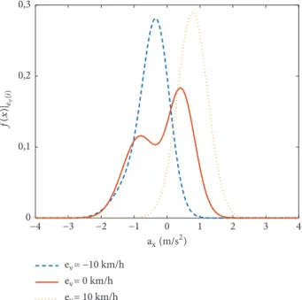
The purpose of the prediction is to predict𝑠1. . . 𝑠𝑛 values based on the probability density function 𝑓(𝑥). For each prediction step𝑖, slices of the function𝑓(𝑥)are generated as 𝑓(𝑥)|𝑒V(𝑖); see, e.g., Figure 6.
The computations ofV𝑥,𝑖 and𝑠𝑖require the value of𝑎𝑥,𝑖, which is generated from the gridding of𝑓(𝑥)|𝑒V(𝑖). The aim
?P= 0 km/h
?P= 10 km/h
?P= −10 km/h 0
0,1 0,2 0,3
−3 −2 −1 0 1 2 3 4
−4
;R(m/M2) f(x)|ev(i)
Figure 6: Slices of probability density function at different velocities.
1MNprediction
2ndprediction
3rdprediction
0 0.2 0.4 0.6 0.8 1 1.2 1.4 1.6
f(MC)
40 60 80 100 120
20
MC(m)
Figure 7: Illustration of the𝑠𝑖probability density function in the predictions.
of the computation is to determine the probability density function of the vehicle position 𝑓(𝑠𝑖), depending on𝑠𝑖 for each time step. The computation is based on the relations of (4a) and (4b), in which the probability density function of𝑓(𝑥)|𝑒V(𝑖) is used. The computation ofV1and𝑠1for𝑖 = 1 requires the deterministic initial velocityV0and position𝑠0, which can be measured.
Due to𝑓(𝑥)|𝑒V(𝑖) the speed and positionsV1,𝑠1are also represented by probability density functions 𝑓(𝑠1), 𝑓(V1).
Therefore, in the computation ofV2, 𝑠2for𝑖 = 2the previous velocity and position of 𝑖 = 1 are considered with their probability density functions. As an illustration, Figure 7 shows an example for𝑖 = 1 . . . 3predictions. Here the initial velocityV𝑥,0 = 140 𝑘𝑚/ℎ, the initial position 𝑠0 = 0, and the sampling time1 𝑠𝑒𝑐are selected. The illustration shows
[m−1]
i
i+1
Li−1 Li Li+1 Li+2 Li+3
si+1
si si+2 si+3 si+4
Ci+1
Ci+2
Ci+3 Ci
s[m]
Figure 8: Piecewise linear formulation of the curvature.
that for𝑖 = 1the probability density function of𝑠1has high values in a small range, which means that the position of the vehicle can be estimated with high probability. However, e.g., for𝑖 = 3the probability density function of𝑠3has high values in a broad range, which means that the forthcoming position of the vehicle has higher uncertainty.
In the prediction of the vehicle position the probability density function has fundamental importance. The probabil- ity𝑃(𝑠𝑖,−< 𝑠𝑖< 𝑠𝑖,+)that the vehicle in the prediction step𝑖is between the positions𝑠𝑖,−. . . 𝑠𝑖,+is computed as follows:
𝑃 (𝑠𝑖,−< 𝑠𝑖< 𝑠𝑖,+) = ∫𝑠𝑖,+
𝑠𝑖,−
𝑓 (𝑠𝑖) 𝑑𝑠𝑖 (5) A safe maneuver to avoid a collision requires a guarantee that the probability of the vehicle in the critical position range 𝑠𝑖,− < 𝑠𝑖 < 𝑠𝑖,+ is smaller than a predefined𝑝𝑚𝑎𝑥 value.
If 𝑃(𝑠𝑖,− < 𝑠𝑖 < 𝑠𝑖,+) > 𝑝𝑚𝑎𝑥, the position 𝑠𝑖,− < 𝑠𝑖 <
𝑠𝑖,+must not be reached by the ego vehicle. Consequently, based on the safe maneuver the vehicle must perform the overtaking or decelerate to the speed of the preceding vehicle.
Thus, the trajectory of the ego vehicle must be designed in such a way that both the estimation of the preceding vehicle motion and the maximum probability level𝑝𝑚𝑎𝑥are taken into consideration. Note that if𝑝𝑚𝑎𝑥is reduced, the safety of the maneuver increases, but the avoidable regions also increase. It can lead to a conservative maneuver, which requires too long traveling in the opposite lane to overtake the preceding vehicle.
Finally, it is necessary to mention that the proposed estimation method is also used for the estimation of the motions of the vehicles in the opposite lane. If the data𝑒V, 𝑎𝑥of the closest vehicle in the opposite lane are available, the prediction of the motion can be performed.
3. Formulation of Trajectory Design
In the overtaking and lane changing strategy the result of the estimation is used for the computation of the vehicle trajectory. In the design two criteria are considered. First,
the results of the estimation must be incorporated in the trajectory design to guarantee safe cruising. Second, the generated trajectory must guarantee a comfortable maneuver.
It means that the motion of the vehicle must be smooth, which is achieved by applying a clothoid trajectory. The advantages of the clothoid trajectory were presented in [22, 23]. In the following an optimal trajectory design method which guarantees both requirements is proposed.
3.1. Modelling of Trajectory Tracking. The lateral motion of the vehicle is formulated based on the kinematic model of the vehicle, such as
𝑑𝑦 (𝑡)
𝑑𝑡 =V𝑥sin𝜓 (𝑡) , (6a) 𝑑𝜓 (𝑡)
𝑑𝑡 = V𝑥
𝐷tan𝛿 (𝑡) , (6b) where 𝑦 is the lateral displacement, V𝑥 is the longitudinal velocity in the vehicle coordinate system,𝜓is the yaw angle, 𝛿is the front steering angle of the front wheels, and 𝐷 is the distance between the front and the rear axle. Translate the motion equation to space domain by making V𝑥 = 𝑑𝑠(𝑡)/𝑑𝑡and assume thatV𝑥is a continuous function in the rearrangement of (6a) and (6b):
𝑑𝑦 (𝑠)
𝑑𝑠 =sin𝜓 (𝑠) (7a)
𝑑𝜓 (𝑠) 𝑑𝑠 =𝛿 (𝑠)
𝐷 . (7b)
The term𝛿(𝑠)/𝐷in (7a) and (7b) represents the curvature𝜅(𝑠) of the path; see also [23].
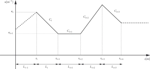
To guarantee a smooth trajectory for the vehicle, the curvature𝜅(𝑠)is constrained so as to generate a clothoid form;
see Figure 8. It leads to the following formulation [23]:
𝜅𝑖+1= 𝜅𝑖+ 𝑐𝑖𝐿𝑖, (8) where𝐿𝑖 = 𝑇V𝑥,𝑖is the distance between two section points and𝑐𝑖is the ratio of the clothoid section.
The motion equations (7a) and (7b) are transformed into a discrete form such as
𝑦𝑖+1= 𝑦𝑖+ 𝐿𝑖sin𝜓 (9a) 𝜓𝑖+1= 𝜓𝑖+ 𝜅𝑖+1𝐿𝑖= 𝜓𝑖+ 𝜅𝑖𝐿𝑖+𝐿2𝑖
2𝑐𝑖 (9b) For small yaw angle differences from the path the assumption sin𝜓 ≈ 𝜓is acceptable.
Using (8), (9a), and (9b) the system is transformed into a state-space representation𝑥𝑖+1 = 𝐴𝑥𝑖+ 𝐵𝑢𝑖in the following way:
[[ [ [
𝑦𝑖+1 𝜓𝑖+1 𝜅𝑖+1
]] ] ]
= [[ [
1 𝐿𝑖 0 0 1 𝐿𝑖 0 0 1 ]] ]
[[ [ 𝑦𝑖 𝜓𝑖 𝜅𝑖 ]] ]
+[[[[ [ 0 𝐿2𝑖 𝐿2𝑖
]] ]] ]
𝑐𝑖 (10)
where the system depends on the values of𝑐𝑖. The purpose of the trajectory computation is to determine these values.
3.2. Optimization of Trajectory Tracking. In the trajectory design the lateral position of the vehicle 𝑦𝑖+1 must be controlled. It is necessary to guarantee that 𝑦𝑖+1 tends to the reference trajectory 𝑦𝑖+1,𝑟𝑒𝑓 as accurately as possible in order to avoid the preceding vehicle and keep the required lanes during the overtaking maneuver. This task leads to a constrained tracking optimization problem, which is formed in the following way.
The trajectory design of the overtaking maneuver is formed in a finite horizon length𝐿𝑛ahead of the vehicle. The lateral position error𝑦𝑖+1−𝑦𝑖+1,𝑟𝑒𝑓in the horizon is described in the following way:
𝑌 (C) = [[ [[ [[ [
𝑦𝑖+1 𝑦𝑖+2 ...
𝑦𝑖+𝑛 ]] ]] ]] ]
− [[ [[ [[ [ [
𝑦𝑖+1,𝑟𝑒𝑓 𝑦𝑖+2,𝑟𝑒𝑓
...
𝑦𝑖+𝑛,𝑟𝑒𝑓 ]] ]] ]] ] ]
= [[ [[ [[ [
𝐶𝐴 𝐶𝐴2 ...
𝐶𝐴𝑛 ]] ]] ]] ]
𝑥𝑖− [[ [[ [[ [
𝑦𝑖+1,𝑟𝑒𝑓 𝑦𝑖+2,𝑟𝑒𝑓
...
𝑦𝑖+𝑛,𝑟𝑒𝑓 ]] ]] ]] ]
+ [[ [[ [[ [ [
𝐶𝐵 0 ⋅ ⋅ ⋅ 0
𝐶𝐴𝐵 𝐶𝐵 ⋅ ⋅ ⋅ 0 ... ... d ...
𝐶𝐴𝑛−1𝐵 𝐶𝐴𝑛−2𝐵 ⋅ ⋅ ⋅ 𝐶𝐵 ]] ]] ]] ] ]
[[ [[ [[ [
𝑐𝑖 𝑐𝑖+1
...
𝑐𝑖+𝑛−1 ]] ]] ]] ]
=A−R+BC
(11)
whereAcontains the current states of the system,Ris built by the reference values,Bis built by the state matrices, and
Cis built by the ratios of clothoid sections. In the tracking problem it is necessary to minimize the following function:
𝐽 (C) = 1
2𝑌𝑇(C) 𝑄𝑌 (C) +C𝑇𝑅C, (12) where𝑄and 𝑅are weighting matrices. The role of𝑄is to minimize the tracking error, while the role of𝑅is to minimize the ratios of the clothoid sections. Substituting (11) into the function (12), the function is transformed as
𝐽 (C) = 1
2(A−R+BC)𝑇𝑄 (A−R+BC) +C𝑇𝑅C= 12(A𝑇−R𝑇+C𝑇B𝑇) 𝑄 (A−R +BC) +C𝑇𝑅C= 1
2(A𝑇𝑄A−A𝑇𝑄𝑅 +A𝑇𝑄BC−R𝑇𝑄A+R𝑇𝑄R−R𝑇𝑄BC +C𝑇B𝑇𝑄A−C𝑇B𝑇𝑄R+C𝑇B𝑇𝑄BC) +C𝑇𝑅C= 12C𝑇(B𝑇𝑄B+ 2𝑅)C+ 12(A𝑇𝑄B
−R𝑇𝑄B)C+C𝑇1
2(B𝑇𝑄A−B𝑇𝑄R) + 𝜀 =1 2
⋅C𝑇𝜙C+ 𝛽𝑇C+C𝑇𝛾 + 𝜀
(13)
where
𝜙 =B𝑇𝑄B+ 2𝑅, (14a)
𝛽𝑇= 1
2(A𝑇𝑄B−R𝑇𝑄B) , (14b)
𝛾 = 1
2(B𝑇𝑄A−B𝑇𝑄R) , (14c)
𝜀 = 1
2(A𝑇𝑄A−A𝑇𝑄𝑅 −R𝑇𝑄A+R𝑇𝑄R) . (14d) In (13) 𝜀 contains all the constant components. Since 𝜀 is independent of the effect ofCon𝐽(C), it can be canceled from the further optimization problem.
Through the minimization of the cost function𝐽(C)the tracking of the reference trajectory𝑦𝑖+1,𝑟𝑒𝑓can be guaranteed.
In order to increase the safety of the maneuver both colli- sion avoidance and lane keeping are built into the design.
Therefore, constraints are incorporated into the trajectory optimization problem. The constraints are related to both the minimum and the maximum values of𝑦𝑖+1. Practically, 𝑦𝑖+1𝑚𝑖𝑛and𝑦𝑖+1𝑚𝑎𝑥are determined by the lanes, which guarantees lane keeping. However, in the overtaking maneuver the constraints must be modified with the current position of the preceding vehicle. The constraints of the minimum values of the positions are formed as𝑦𝑖+𝑗 ≥ 𝑦𝑖+𝑗𝑚𝑖𝑛,𝑗 ∈ {1, 𝑛}. The inequalities are transformed into a matrix representation:
A+BC≥ 𝑌𝑚𝑖𝑛, (15)
ego vehicle overtaken vehicle
opposite vehicle
0
ysafety
ysafety ymin
ymax
Figure 9: Determination of𝑌𝑚𝑖𝑛and𝑌𝑚𝑎𝑥.
where𝑌𝑚𝑖𝑛 = [𝑦𝑚𝑖𝑛𝑖+1 𝑦𝑖+2𝑚𝑖𝑛 ⋅ ⋅ ⋅ 𝑦𝑖+𝑛𝑚𝑖𝑛]𝑇. Thus, the constraint on the clothoid ratiosCis formed as
A− 𝑌𝑚𝑖𝑛≥ −BC. (16)
Similarly, the constraints of the maximum values of𝑦𝑖+1are derived as
𝑌𝑚𝑎𝑥−A≥BC, (17)
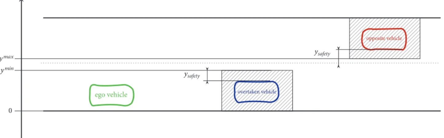
where𝑌𝑚𝑎𝑥= [𝑦𝑖+1𝑚𝑎𝑥 𝑦𝑖+2𝑚𝑎𝑥 ⋅ ⋅ ⋅ 𝑦𝑚𝑎𝑥𝑖+𝑛 ]𝑇. The minimum𝑌𝑚𝑖𝑛 and maximum𝑌𝑚𝑎𝑥values are determined by the edges of the lanes and the surrounding vehicles, especially the preceding vehicle and the vehicle in the opposite lane. If a vehicle in the opposite lane performs a lane change maneuver, it can limit the lateral motion of the ego vehicle. This information is also incorporated in𝑌𝑚𝑎𝑥, with which the safe cruising of the ego vehicle is guaranteed against collisions with the vehicles from the opposite lane. The selections of𝑌𝑚𝑖𝑛and𝑌𝑚𝑎𝑥are illustrated in Figure 9, where𝑦𝑠𝑎𝑓𝑒𝑡𝑦describes a safety zone of the vehicles.
Finally, from (13), (16), and (17) the constrained trajectory optimization problem is formed as
𝑢𝑖min...𝑢𝑖+𝑛−1
1
2C𝑇𝜙C+ 𝛽𝑇C+C𝑇𝛾 (18) such that the following constraints are also guaranteed:
A− 𝑌𝑚𝑖𝑛≥ −BC (19a)
𝑌𝑚𝑎𝑥−A≥BC (19b)
C∈C (19c)
where Ccontains the achievable clothoid ratios. The opti- mization problem can be solved using standard quadratic programming methods, e.g., [24, 25]. The solution of (18) leads to a series of clothoid ratios on the horizon𝐿𝑛. The current ratio𝑐𝑖can be computed online during the cruising of the vehicle.
3.3. Decision Strategy of Overtaking and Lane Changing. The overtaking and lane changing strategy is based on the con- strained trajectory optimization method (18). Although the constraints and the achievable clothoid ratios are considered, the calculated tracking must be modified for safety reasons.
Before the maneuver the ego vehicle reaches a preceding vehicle which is traveling at a slower speed. The vehicle must follow the preceding vehicle. If the preceding vehicle accelerates or decelerates the ego vehicle must strictly track the velocity within the speed limit. Meanwhile, it calculates a safe trajectory for the overtaking and lane changing. The optimization method (18) results in a clothoid curve, which guarantees the cruising of the ego vehicle between the minimum and the maximum limits.
However, if there is a follower vehicle in the inner lane which is traveling at a higher velocity, a conflict with the ego vehicle may occur during the overtaking maneuver.
Moreover, if there is a vehicle in the opposite lane, a conflict with the ego vehicle in the maneuver may also occur. These maneuvers are considered unfeasible. Infeasibility means that it is impossible to find an appropriate trajectory which guarantees both the minimization (18) and the constraints (19a), (19b), and (19c). In this case the ego vehicle must follow the preceding vehicle and modify the longitudinal dynamics.
When the traffic situation changes and the optimization becomes feasible, the overtaking maneuver can be performed.
The maneuver is realized through the actuation of steering and driving/braking systems; see, e.g., [26].
Note that the proposed method can be used not only for overtaking, but also for simple lane changing maneuvers, e.g., changing the route in a highway intersection. In this scenario the reference signal of the road 𝑦𝑖+1,𝑟𝑒𝑓 must be modified according to the parameters of the requested lane.
Moreover, in a lane changing maneuver the constraints𝑌𝑚𝑖𝑛 and𝑌𝑚𝑎𝑥must be modified for the new lane. Furthermore, the proposed optimization (18) and decision problem can be formed as a MPC task, in which the steering intervention can also be incorporated. However, the entire control system must guarantee the robustness of the system, which can lead to high complexity in the computation of the vehicle control. In the paper a robust LPV-based control design method is proposed
G()
K() u
yref
ref
Wz,1 Wr,1
Wr,2
Wz,2 Wz,3
Ww,2 Ww,1
e,a ey,a
z1 z3
z2
w1 w2
Figure 10: Closed-loop interconnection structure.
to guarantee the tracking of the generated trajectory and the robustness of the controlled system.
4. Robust LPV Control for Autonomous Overtaking
The goal of the robust LPV control is to guarantee the tracking of the trajectory, which has been generated by optimization (18) together with the decision algorithm. The results of the optimization are𝑢𝑖. . . 𝑢𝑖+𝑛−1, which are equal to the ratios of the clothoid sections𝑐𝑖. . . 𝑐𝑖+𝑛−1. In the case of the tracking control the vehicle must follow the reference path 𝑦𝑟𝑒𝑓 = 𝑦𝑖+1 = 𝑦1and the reference heading angle𝜓𝑟𝑒𝑓= 𝜓𝑖+1 = 𝜓1. The reference signals are computed from (10) such as
𝑦𝑟𝑒𝑓= 𝑦0+ 𝐿0𝜓0 (20a) 𝜓𝑟𝑒𝑓= 𝜓0+ 𝐿0𝜅0+𝐿20
2 𝑐0 (20b)
where𝑦0, 𝜓0are related to𝑦(𝑡), 𝜓(𝑡)in discrete time, while𝐿0 is the length of the forthcoming segment and𝜅0is the result in the previous trajectory computation step. The parameter𝑐0 is the first element among the results of the optimization𝑢0.
After the computation of the reference signals the track- ing performances together with the control performance are defined as
𝑧1= 𝑦𝑟𝑒𝑓− 𝑦 (𝑡) 𝑧1 → 𝑚𝑖𝑛, (21a) 𝑧2= 𝜓𝑟𝑒𝑓− 𝜓 (𝑡) 𝑧2 → 𝑚𝑖𝑛, (21b) 𝑧3= 𝛿 (𝑡) 𝑧3 → 𝑚𝑖𝑛. (21c) The performance vector is as follows:𝑧 = [𝑧1 𝑧2 𝑧3]𝑇.
The model of the vehicle is described by the dynamical bicycle model; see [27]:
𝑚 ̈𝑦 = 𝐶𝑓(𝛿 − ̇𝜓𝑙𝑓+ ̇𝑦
V𝑥 ) + 𝐶𝑟( ̇𝜓𝑙𝑟− ̇𝑦
V𝑥 ) (22a)
𝐽 ̈𝜓 = 𝐶𝑓𝑙𝑓(𝛿 − ̇𝜓𝑙𝑓+ ̇𝑦
V𝑥 ) − 𝐶𝑟𝑙𝑟( ̇𝜓𝑙𝑟− ̇𝑦
V𝑥 ) (22b)
where𝐽is the yaw inertia of the vehicle,𝑚is the vehicle mass, 𝐶𝑓, 𝐶𝑟 are the cornering stiffness coefficients, and𝑙𝑓, 𝑙𝑟 are geometric parameters. The signal ̇𝑦is the lateral velocity and
̇𝜓is the yaw rate. The longitudinal velocityV𝑥may vary along the route of the vehicle; therefore it is chosen as a scheduling variable. Equations (22a) and (22b) can be transformed into a state-space representation, where the state vector is 𝑥 = [ ̇𝜓 ̇𝑦 𝜓 𝑦]𝑇, the control input is the steering angle𝑢 = 𝛿, and the measured output vector is𝑦𝑚 = [𝜓 𝑦]𝑇. The state equation and the performances as well as the measurements are written as
̇𝑥 = 𝐴 (𝜌) 𝑥 + 𝐵𝑢 (23a)
𝑧 = 𝐶1𝑥, (23b)
𝑦𝑚= 𝐶2𝑥 + 𝐷𝑢, (23c) where𝜌 =V𝑥is selected as a scheduling variable. Its value is modified through the decision strategy.
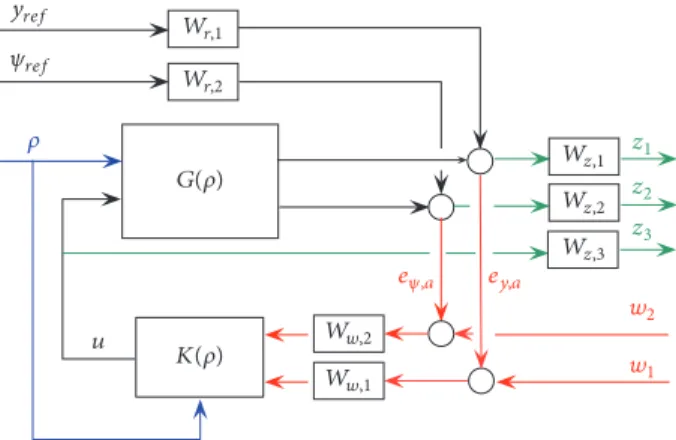
The control design is based on a weighting strategy, which is formulated through a closed-loop interconnection struc- ture; see Figure 10. The interconnection structure contains several weighting functions, whose roles are to guarantee the trade-off between the performances and to scale the signals.
The weights𝑊𝑤,1, 𝑊𝑤,2are related to the sensor characteris- tics on the lateral error and yaw error measurement. These weights are related to the sensor dynamics. 𝑊𝑧,1, 𝑊𝑧,2, and 𝑊𝑧,3 are the weights for the performances, which represent the minimization of𝑧1, 𝑧2, and𝑧3. The weights are formed as 𝑊𝑧,𝑖= 𝐴𝑖/(𝑇𝑖𝑠 + 1)where𝐴𝑖, 𝑇𝑖are design parameters. These parameters influence the balance between the performances 𝑧1, 𝑧2, and 𝑧3. Moreover, the role of the weight 𝑊𝑟,𝑖 is to consider the dynamics of the reference signals𝑦𝑟𝑒𝑓, 𝜓𝑟𝑒𝑓. The blocks also represent the dynamics of their variations.
The design of the control is based on robust LPV methods.
The advantage of these methods is that the controller meets stability and performance demands by using affine parame- terized Lyapunov functions in the entire operational interval, since the controller is able to adapt to the current operational conditions; see [28, 29]. The solution of an LPV problem is governed by the set of infinite dimensional LMIs being satisfied for all 𝜌 ∈ FP; thus it is a convex problem. In
(a) Start of overtaking
(b) End of overtaking
(c) Approaching the preceding vehicle
(d) Tracking the preceding vehicle
(e) Change of lane
(f) Cruising with its own reference velocity Figure 11: Simulation scenario.
practice, this problem is set up by gridding the parameter space and solving the set of LMIs that hold on the subset of FP. The inducedL2 norm of parameter-dependent stable LPV systems with zero initial conditions is defined as
inf𝐾 sup
∈FP
sup
‖𝑤‖2 ̸=0,𝑤∈L2
‖𝑧‖2
‖𝑤‖2, (24)
where 𝑤is the disturbance and𝑧 is the performance. The result of the optimization is the steering angle𝛿.
5. Simulation Results
To illustrate the efficiency of the proposed method a complex simulation scenario is presented. The traffic scenario contains
reference real
−6
−5
−4
−3
−2
−1 0 1 2 3 4
Lateral position (m)
100 200 300 400 500 600 700 800 0
Station (m)
(a) Trajectory of the vehicle
80 85 90 95 100 105 110 115 120
Speed (km/h)
100 200 300 400 500 600 700 800 0
Station (m)
(b) Velocity profile Figure 12: Simulation results.
four vehicles, such as the ego vehicle, two preceding vehicles, and another vehicle in the opposite lane. In the setting of the optimal trajectory computation the sample time is set at 𝑇 = 0.1𝑠with𝑛 = 20the prediction points. The simulation is performed using the high-complexity vehicle dynamic software CarSim.
The simulation is illustrated in Figure 11. At the beginning of the simulation the ego vehicle (blue) reaches the preced- ing vehicle (white) due to the significant difference in the velocities; see Figure 11(a). Since the overtaking maneuver is feasible, it is carried out as Figure 11(b) shows. Then the ego vehicle reaches the next preceding vehicle (green), which also has lower velocity; see Figure 11(c). The ego vehicle calculates the overtaking trajectory based on the optimization task (18) and the constraints𝑌𝑚𝑖𝑛and𝑌𝑚𝑎𝑥(19a), (19b), and (19c). But there is a vehicle in the opposite lane (red), which makes the overtaking maneuver unfeasible. Thus, the ego vehicle must follow the preceding vehicle, which results in the reduction of its velocity; see Figure 11(d). Finally, the ego vehicle performs a lane changing in order to modify its route at an exit ramp.
In this case a new reference signal𝑦𝑖+1,𝑟𝑒𝑓is set as shown in Figure 11(e). Then the velocity of the vehicle increases; see Figure 11(f).
The numerical values of the lateral position and the velocity are illustrated in Figure 12. The increase and decrease of the lateral positions at 100 𝑚 and 200 𝑚, respectively, illustrate the overtaking of the first slower vehicle (white) and then the tracking of the second preceding vehicle (green) due to the third vehicle (red) coming from the opposite lane;
see Figure 12(a). In the proposed scenario the safe distance between the vehicles is 20𝑚, which has been kept by the ego vehicle. The initial velocity is110 𝑘𝑚/ℎ, which must be reduced to keep the velocity of the green preceding vehicle (90𝑘𝑚/ℎ); see Figure 12(b). At 500 𝑚 the lane change is carried out, which results in the changes of the lateral position and the increases in the velocity compared to the original value.
6. Conclusions
In the paper an overtaking and a lane changing strategy have been proposed. The expected motion of the preceding vehicle is predicted by using clustering methods and probability density functions. The trajectory design is formed as a constrained optimization problem, in which the traffic in the lanes of the road is considered. In the decision mak- ing concerning overtaking the motions of the surrounding vehicles such as the follower vehicle with higher velocity and vehicles in the opposite lane is also incorporated. The robust parameter varying tracking control design of the lateral dynamics has been presented. The proposed strategy is able to guarantee the safe motion of the vehicles and handle the interactions with the other traffic participants. The results have been illustrated through simulation examples.
Data Availability
No data were used to support this study.
Conflicts of Interest
The authors declare that they have no conflicts of interest.
Acknowledgments
The research reported in this paper was supported by the Higher Education Excellence Program of the Ministry of Human Capacities within the frame of Artificial Intelligence research area of Budapest University of Technology and Economics (BME FIKPMI/FM). The research was supported by the Hungarian Government and cofinanced by the Euro- pean Social Fund through the project ”Talent Management in Autonomous Vehicle Control Technologies” (EFOP-3.6.3- VEKOP-16-2017-00001). The work of Bal´azs N´emeth was partially supported by the J´anos Bolyai Research Scholarship
of the Hungarian Academy of Sciences and the ´UNKP-18-4 New National Excellence Program of the Ministry of Human Capacities.
References
[1] T. Shamir, “How should an autonomous vehicle overtake a slower moving vehicle: design and analysis of an optimal trajectory,”Institute of Electrical and Electronics Engineers Trans- actions on Automatic Control, vol. 49, no. 4, pp. 607–610, 2004.
[2] K. Berntorp, “Path planning and integrated collision avoidance for autonomous vehicles,” inProceedings of the 2017 American Control Conference, ACC 2017, pp. 4023–4028, USA, May 2017.
[3] N. Murgovski and J. Sjoberg, “Predictive cruise control with autonomous overtaking,” inProceedings of the 2015 54th IEEE Conference on Decision and Control (CDC), pp. 644–649, Osaka, December 2015.
[4] N. A. Nguyen, D. Moser, P. Schrangl, L. del Re, and S. Jones,
“Autonomous overtaking using stochastic model predictive control,” inProceedings of the 2017 11th Asian Control Conference (ASCC), pp. 1005–1010, Gold Coast, QLD, December 2017.
[5] F. Molinari, N. N. Anh, and L. Del Re, “Efficient mixed integer programming for autonomous overtaking,” inProceedings of the 2017 American Control Conference, ACC 2017, pp. 2303–2308, USA, May 2017.
[6] J. E. Naranjo, C. Gonz´alez, R. Garc´ıa, and T. De Pedro, “Lane- change fuzzy control in autonomous vehicles for the overtaking maneuver,” IEEE Transactions on Intelligent Transportation Systems, vol. 9, no. 3, pp. 438–450, 2008.
[7] D. C. K. Ngai and N. H. C. Yung, “A multiple-goal reinforcement learning method for complex vehicle overtaking maneuvers,”
IEEE Transactions on Intelligent Transportation Systems, vol. 12, no. 2, pp. 509–522, 2011.
[8] V. Milan´es, D. F. Llorca, J. Villagr´a et al., “Intelligent automatic overtaking system using vision for vehicle detection,”Expert Systems with Applications, vol. 39, no. 3, pp. 3362–3373, 2012.
[9] G. Usman and F. Kunwar, “Autonomous vehicle overtaking - An online solution,” inProceedings of the 2009 IEEE International Conference on Automation and Logistics, ICAL 2009, pp. 596–
601, China, August 2009.
[10] P. Petrov and F. Nashashibi, “Modeling and nonlinear adaptive control for autonomous vehicle overtaking,”IEEE Transactions on Intelligent Transportation Systems, vol. 15, no. 4, pp. 1643–
1656, 2014.
[11] A. Carvalho, S. Lef´evre, G. Schildbach, J. Kong, and F. Borrelli,
“Automated driving: the role of forecasts and uncertainty—a control perspective,”European Journal of Control, vol. 24, pp.
14–32, 2015.
[12] S. Lef`evre, D. Vasquez, and C. Laugier, “A survey on mo- tion prediction and risk assessment for intelligent vehicles,”
ROBOMECH Journal, vol. 1, no. 1, 2014.
[13] T. Gindele, S. Brechtel, and R. Dillmann, “A probabilistic model for estimating driver behaviors and vehicle trajectories in traffic environments,” inProceedings of the 13th International IEEE Conference on Intelligent Transportation Systems (ITSC ’10), pp.
1625–1631, IEEE, Funchal, Portugal, September 2010.
[14] M. Althoff and A. Mergel, “Comparison of Markov chain abstraction and Monte Carlo simulation for the safety assess- ment of autonomous cars,” IEEE Transactions on Intelligent Transportation Systems, vol. 12, no. 4, pp. 1237–1247, 2011.
[15] K. Okamoto, K. Berntorp, and S. Di Cairano, “Similarity-based vehicle-motion prediction,” inProceedings of the 2017 American Control Conference, ACC 2017, pp. 303–308, USA, May 2017.
[16] R. Kala and K. Warwick, “Motion planning of autonomous vehicles in a non-autonomous vehicle environment without speed lanes,”Engineering Applications of Artificial Intelligence, vol. 26, no. 5-6, pp. 1588–1601, 2013.
[17] L. Kaufman and P. Rousseeuw,Finding Groups in Data: An Introduction to Cluster Analysis, John Wiley & Sons, New York, NY, USA, 1990.
[18] S. Guha, R. Rastogi, and K. Shim, “CURE: An efficient clustering algorithm for large databases,” in Proceedings of the ACM SIGMOD International Conference on Management of Data, pp.
73–84, 1998.
[19] M. Ester, H.-P. Kriegel, J. Sander, and X. Xu, “A density-based algorithm for discovering clusters in large spatial databases with noise,” inProceedings of the in 2nd Intenational Conference Knowledge Discovery and Data Mining, pp. 226–231, Portland, 1996.
[20] H. S. Park, J. Lee, and C. Jun, “A k-meanslike algorithm for k- medoids clustering and its performance,” inProceedings of the ICCIE, 2006.
[21] T. M. Kodinariya and P. R. Makwana, “Review on determining number of cluster in K-means clustering,”International Journal of Advance Research in Computer Science and Management Studies, vol. 1, pp. 90–95, 2013.
[22] D. K. Wilde, “Computing clothoid segments for trajectory generation,” inProceedings of the 2009 IEEE/RSJ International Conference on Intelligent Robots and Systems, IROS 2009, pp.
2440–2445, October 2009.
[23] P. F. Lima, M. Trincavelli, J. Martensson, and B. Wahlberg,
“Clothoid-based model predictive control for autonomous driv- ing,” in proceedings of the European Control Conference, pp.
2983–2990, 2015.
[24] P. E. Gill, W. Murray, and M. H. Wright,Practical Optimization, Academic Press, 1981.
[25] C. Schmid and L. T. Biegler, “Quadratic programming methods for reduced hessian SQP,”Computers & Chemical Engineering, vol. 18, no. 9, pp. 817–832, 1994.
[26] P. G´asp´ar and B. N´emeth, “Integrated control design for driver assistance systems based on LPV methods,”International Journal of Control, vol. 89, no. 12, pp. 2420–2433, 2016.
[27] R. Rajamani,Vehicle Dynamics and Control, Springer, New York, NY, USA, 2012.
[28] F. Wu, X. H. Yang, A. Packard, and G. Becker, “InducedL2-norm control for LPV systems with bounded parameter variation rates,”International Journal of Robust and Nonlinear Control, vol. 6, no. 9-10, pp. 983–998, 1996.
[29] J. Yu and A. Sideris, “H∞control with parametric Lyapunov functions,”Systems & Control Letters, vol. 30, no. 2-3, pp. 57–
69, 1997.
International Journal of
Aerospace Engineering
Hindawi
www.hindawi.com Volume 2018
Robotics
Journal ofHindawi
www.hindawi.com Volume 2018
Hindawi
www.hindawi.com Volume 2018
Active and Passive Electronic Components VLSI Design
Hindawi
www.hindawi.com Volume 2018
Hindawi
www.hindawi.com Volume 2018
Shock and Vibration
Hindawi
www.hindawi.com Volume 2018
Civil Engineering
Advances inAcoustics and VibrationAdvances in
Hindawi
www.hindawi.com Volume 2018
Hindawi
www.hindawi.com Volume 2018
Electrical and Computer Engineering
Journal of
Advances in OptoElectronics
Hindawi
www.hindawi.com Volume 2018
Hindawi Publishing Corporation
http://www.hindawi.com Volume 2013
Hindawi www.hindawi.com
The Scientific World Journal
Volume 2018
Control Science and Engineering
Journal of
Hindawi
www.hindawi.com Volume 2018
Hindawi www.hindawi.com
Journal of
Engineering
Volume 2018
Sensors
Journal ofHindawi
www.hindawi.com Volume 2018
Machinery
Hindawi
www.hindawi.com Volume 2018
Modelling &
Simulation in Engineering
Hindawi
www.hindawi.com Volume 2018
Hindawi
www.hindawi.com Volume 2018
Chemical Engineering
International Journal of Antennas and
Propagation
International Journal of
Hindawi
www.hindawi.com Volume 2018
Hindawi
www.hindawi.com Volume 2018
Navigation and Observation
International Journal of
Hindawi
www.hindawi.com Volume 2018