Graph-based Multi-Vehicle Overtaking Strategy for
Autonomous Vehicles
Tam´as Heged˝us∗,Bal´azs N´emeth∗∗,P´eter G´asp´ar∗∗
∗ Department of Control for Transportation and Vehicle Systems, Budapest University of Technology and Economics, Stoczek u. 2, H-1111 Budapest, Hungary. E-mail: hegedus.tamas@mail.bme.hu
∗∗ Institute for Computer Science and Control, Hungarian Academy of Sciences, Kende u. 13-17, H-1111 Budapest, Hungary.
E-mail: [balazs.nemeth;peter.gaspar]@sztaki.mta.hu
Abstract: The paper proposes an advanced graph-based optimal solution to overtaking scenarios for autonomous vehicles. The advantage of the method is that it is possible to consider several human-driven vehicles in the environment of autonomous vehicles. There is a probability- based approach in the background of the graph-based route selection optimization, with which the motions of the human-driven vehicles are predicted. The result of the method is the road and the velocity profile of the autonomous vehicle, with which emergencies and even collisions can be avoided. The efficiency of the optimization algorithm is illustrated through a simulation scenario.
Keywords: autonomous vehicles, overtaking strategy, graph-based route selection, motion prediction
1. INTRODUCTION AND MOTIVATION Overtaking is one of the most risky maneuvers for drivers due to the high velocity of the participants and many unexpected events and uncertainties of the maneuver. For example, in 2015, 9,055 vehicles were involved in overtak- ing accidents in Great Britain (RoSPA [2017]), while the total number of reported deaths was 1,730 and the number of seriously injured people was 22,144, see Lloyd et al.
[2016]. Since overtaking maneuvers are a salient cause of accidents, crucial goal of autonomous vehicle control is to design a strategy with which emergency situations can be avoided. It requires the motion prediction of the human- driven vehicles, which must be incorporated in the road and velocity design of autonomous vehicles.
In the field of overtaking control of autonomous vehicles several different approaches have been developed. The advantage of the Model Predictive Control (MPC)-based approaches is that they consider the prediction about
? The research was supported by the Hungarian Government and co- financed by the European Social Fund through the project ”Talent management in autonomous vehicle control technologies” (EFOP- 3.6.3-VEKOP-16-2017-00001).
The research reported in this paper was supported by the Higher Education Excellence Program of the Ministry of Human Capacities in the frame of Artificial Intelligence research area of Budapest University of Technology and Economics (BME FIKPMI/FM).
The work of Bal´azs N´emeth was partially supported by the J´anos Bolyai Research Scholarship of the Hungarian Academy of Sciences and the ´UNKP-18-4 New National Excellence Program of the Min- istry of Human Capacities.
the surrounding vehicles in the design of the current in- tervention. For example, in Berntorp [2017] a technique for path planning together with collision avoidance with the application of overtaking was found. Murgovski and Sj¨oberg [2015] proposed a predictive control scheme for overtaking problems, which was solved through a convex optimization method. Similarly, Moser et al. [2017] pro- posed the use of a mixed integer programming problem in the context of MPC. The advantage of this viewpoint was to consider the switching in the control problem.
Moreover, in the method the surrounding vehicles were considered through stochastic approaches. Another mixed integer programming method was proposed in Molinari et al. [2017], with which the complexity of the computation and the number of variables were reduced. An autonomous overtaking problem was presented from the viewpoint of stochastic processes in Nguyen et al. [2017]. The core of this method was to predict the longitudinal and lateral velocities of the surrounding vehicles, while the overtaking was solved through a stochastic predictive control. Petrov and Nashahibi [2014] presented a nonlinear adaptive con- troller for a two-vehicle automated overtaking maneuver, in which the problem was formed as a tracking task.
Although the derived method led to the implementation of the nonlinear control with low computation efforts, only two vehicles in the overtaking maneuver were incorpo- rated.
Vehicle motion prediction is strongly linked to the overtak- ing problem of autonomous vehicles, see Carvalho et al.
[2015]. Therefore, several methods were devised to es-
timate the future intentions and motion of the human drivers (Lefevre et al. [2014]). Probabilistic approaches based on the Dynamic Bayesian Network and Markov chain models were found in Gindele et al. [2010], Althoff and Mergel [2011], Firl and Tran [2011]. Furthermore, Okamoto et al. [2017] proposed a method which used the past similarities in the vehicle motion between the actual vehicle and a predefined number of test vehicles. The factor of driver aggression and the motion of vehicles in an unorganized traffic in the motion planning of overtaking maneuver were considered in Kala and Warwick [2013].
Simultaneously, the overtaking behaviour of the human driver was considered in the control design of Milan´es et al. [2012]. Thus, different trajectories were generated depending on the characteristics of the vehicle. In this approach the surrounding vehicles were detected through a stereo vision system.
In this paper the proposed solution to the overtaking problem is based on an optimization over a graph. The advantage of the method is that it is sufficiently uni- versal to consider multi-vehicle overtaking scenarios. The paper proposes the prediction of the surrounding vehicles through a probability-based approach, in which the predic- tions of the longitudinal and lateral motions of the vehicles are combined. A graph search algorithm is proposed using the Dijkstra method, which is often used in autonomous vehicle applications for navigation in urban areas, see e.g.
Gonz´alez et al. [2016]. As a novelty, in this paper the graph search method is proposed for the combination of the road and velocity selection of the overtaking maneuver.
The structure of the paper is the following. The predic- tion of the motion of the human-driven vehicles through probability-based methods is formed in Section 2. Based on the result of the prediction a graph-based decision algorithm is built, as proposed in Section 3. Section 4 demonstrates the efficiency of the method through a mul- tiple vehicle scenario in the CarSim simulation system.
Finally, the results of the paper are concluded in Section 5.
2. THE PREDICTION OF THE SURROUNDING HUMAN-DRIVEN VEHICLE MOTION
Since there can be several overtaking interactions between the autonomous and the human-driven vehicles, the au- tonomous vehicle requires information about the inten- tions of the human-driven vehicles. If Vehicle-to-Vehicle communication technology among vehicles is available, considerable information about the human-driven to the autonomous vehicle can be transmitted, e.g. velocity or acceleration signals. However, these signals do not provide enough information about the forthcoming intentions of the vehicle, e.g. about the starting time of the overtaking maneuver. Moreover, the intentions depend on the habit and the capability of the driver, which may vary in each hu- man. Therefore, the prediction of the surrounding human- driven vehicle motion has been built on a probability-based approach. In the following the prediction is divided into lateral and longitudinal examinations, which are finally combined together.
Lateral motion prediction
The prediction method of the lateral motion considers that the path of the vehicle can be modeled as a clothoid curve, which is sufficiently smooth to guarantee the comfort per- formances of the human driver. The path is divided into four clothoid sections with similar parameters. The compu- tation of the lateral accelerationalatduring the maneuver is proposed in Wilde [2009]. Through the formulation of alatthe trajectories of the vehicle atv0initial velocity are generated.
The probability of the vehicle overtaking motion is de- scribed by a Gamma distribution (Xu et al. [2015]). The probability density function is formed as
flat(x, α, β) = βαxα−1e−βx
Γ(α) , (1)
where x > 0 and α > 0 are the shape parameters and β >0 is the rate parameter. The gamma function Γ(α) in the denominator is formed as
Γ(α) =
∞
Z
0
xα−1e−xdx. (2)
For α ∈ N the gamma function is simplified to the expression Γ(α) = (α−1)!
Based on equation (1) the probability of the maneuver in the acceleration range [alat,min, alat,max] is computed as
Plat(alat,min,alat,max) =
alat,max
Z
alat,min
flat(x)dx=
=Plat(alat,max)−Plat(alat,min), (3) where f(x) = f(x, α, β) for fixed α, β parameters. Since there is an F relationship between the lateral accelera- tion alat and the lateral displacement y of the vehicle alat=F(y) (Rajamani [2005]), the probability can be also expressed as
Plat(ymin, ymax) =
ymax
Z
ymin
flat(z)dz=
=Plat(ymax)−Plat(ymin), (4) where ymin and ymax are the bounds of the lateral dis- placement range. Note that in the bounds it is necessary to consider the half width of the vehicle chassis, which increases the covered area of the vehicle on the road during the maneuver.
Longitudinal motion prediction
Since the velocity of the vehicle can be modified through its cruising by the driver, it must be incorporated in the prediction of the human-driven vehicle motion. The prediction is based on a time horizon T, which depends on the current speed of the human-driven vehicle v0. It is divided intonnumber of equidistant time segmentstk, which results inti =
i
P
k=1
tk fori = 1. . . n. The predicted distance of the vehiclesi is formed as
si=s0+v0ti+1
2alongt2i, (5)
where s0, v0 are the current position and velocity of the vehicle and the acceleration along is considered to be constant. However, the driver is able to select a ∈[along,min, along,max], where |along,min|= |along,max|, which has a normal distribution. The probability density function is defined as
flong(x) = 1 σ√
2πe−(x−µ)22σ2 , (6)
whereσandµare the deviation and the mean of the pro- cess. Thus, the probability of the acceleration maneuver with a givenalong∈[along,min, along,max] is
Plong(si(ti), sj(tj)) =
sj(tj)
Z
si(ti)
flong(x)dx. (7)
Combined prediction
Since the lateral and the longitudinal motions of the human-driven vehicle can be performed simultaneously, the probability of the combined maneuver must be pre- dicted. However, it must be characterized by probabil- ity, whether the driver selects the overtaking or the ap- proaching to a leading vehicle. Its probability is expressed through a sigmoid function, see Wissing et al. [2017]
Pdec(λ) = 1
1 +e−mλ, (8)
where m represents the steepness of the curve and λ is defined as
λ= vprec−v0
d , (9)
where d is the distance between the vehicles,vprec is the velocity of the leading vehicle andv0is the current velocity of the examined vehicle. The sigmoid function represents that if λ= 0 then the probability of the beginning of the overtaking maneuver is 50%. Ifλ <0 then the willingness for overtaking is reduced, while atλ >0 the overtaking is more probable. Farah et al. [2009] provided the support for the selection of m. It proposes that the drivers generally start the overtaking maneuver when the distance of the following vehicle from the leading vehicle is 1.5s, which results ind= 1.5|vprec−v0|.
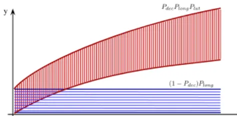
Since the driver has the possibility to decide about the overtaking maneuver, the probability of the combined longitudinal-lateral motion has two components. Both of them are expressed as geometric probabilities, as illus- trated in Figure 1. First, the leading vehicle can be driven straightforward, whose probability is 1−Pdec(λ). In this way the vehicle covers the road in the longitudinal straight direction with probability Plong(si(ti), sj(tj)). In the lat- eral direction the probability is determined by the width of the vehicle, which is 1. Thus, the combined probability is
(1−Pdec(λ))Plong(si(ti), sj(tj)). (10) Second, the driver can decide about the start of the overtaking maneuver, which is represented byPdec(λ). In this case the probability of the lateral motion is expressed through Plat(ymin, ymax), which results in the combined probability
Pdec(λ)Plong(si(ti), sj(tj))Plat(ymin, ymax). (11)
Finally, it is necessary to sum up the probability values of the two components, such as
P(λ, si(ti), sj(tj), ymin, ymax) =
= (1−Pdec(λ))Plong(si(ti), sj(tj))+
+Pdec(λ)Plong(si(ti), sj(tj))Plat(ymin, ymax). (12) The probability can be computed to all time segments between ti, tj. It ensures that the vehicle is positioned betweensi, sj, its longitudinal position has a normal dis- tribution, the lateral position has a Gamma distribution, considering the probability of the beginning of the over- taking maneuver. It results in a map for the examined human-driven vehicle, which provides information about the probability of the forthcoming positioning.
(1−Pdec)Plong PdecPlongPlat
x y
Fig. 1. Illustration of the probability computation forP 3. GRAPH-BASED ROUTE SELECTION
ALGORITHM
The goal of this section is to find the route of the au- tonomous vehicle which results in the minimum proba- bility of a collision. During the design it is necessary to consider all of the human-driven vehicles, which are in the environment of the controlled vehicle. Moreover, it is necessary to define the probability of a collision, whose minimization along the route of the vehicle is the objective.
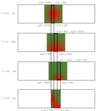
The determination method of the collision probability from the prediction of the vehicles is illustrated in Figure 2.
The predicted positionsh from (5) of the leading human- driven vehicle is illustrated in the coloured rectangle, in which red represents the high probability of the vehicle position, while green is related to the low probability.
In the example the prediction is computed for three time segments with tj − ti = 0.5s length, as shown the upper three blocks in Figure 2. The probabilities P(λ, si(ti), sj(tj), ymin, ymax) in the areas are computed through (12).
Moreover, the probability of the collision depends on the motion of the autonomous vehicle. In the case of the controlled vehicle it is necessary to determine the longitudinal position of the vehicle between ti and tj. In Figure 2 these areas are represented by the rectangles with black edges in the upper three blocks. The longitudinal positions of the vehicle inti, tj are computed as
sa=sa,0+va,0tz+1
2aat2z z={i, j}, (13) wheresa,0, va,0are the current position and velocity of the autonomous vehicle andaais the longitudinal acceleration command. Note that the prediction of the lateral position of the autonomous vehicle is unnecessary, because it results from the graph-based route selection algorithm, together with the acceleration commandaa.
The map about the probability of a collision is generated through the intersection areas of the human-driven predic- tion and the autonomous vehicle motion in the different ti, tj times. The set-up of the map about the probability of a collision is illustrated in the last block of Figure 2.
t= 2.5. . .3s
t= 3. . .3.5s
t= 3.5. . .4s
t= 2.5. . .4s
sh(t= 2.5s) sh(t= 3s) sa(t= 2.5s). . . sa(t= 3s)
sh(t= 3.5s) sh(t= 3s)
sh(t= 3.5s) sh(t= 4s) sa(t= 3s). . . sa(t= 3.5s)
sa(t= 3.5s). . . sa(t= 4s)
sa(t= 2.5s). . . sa(t= 4s)
Fig. 2. Illustration of the computation of collision proba- bility
In multiple vehicle scenarios it is necessary to determine the areas of P(λ, si(ti), sj(tj), ymin, ymax) for all human- driven vehicles. Since the probability of a collision Pc
increases with the number of human-driven vehicles, each probability from the prediction must be summed up, such as
Pc(ti, tj) =
N
X
l=1
P(λ, si(ti), sj(tj), ymin, ymax)
N , (14)
where N is the number of human-driven vehicles in the region of interest. The division with N guarantees that the value of Pc(ti, tj) is between 0 and 1.
The following examples in Figure 3 presents the results of the Pc(ti, tj) for a 300 m long horizon. In the figures the pale green colour represents the low risk of a collision, while the red colour is related to the high risk of a collision.
In the first scenario of the example the longitudinal veloc- ity of the leading vehicle is 26m/s, while the velocity of the following autonomous vehicle is 28 m/s, see Figure 3(a).
The current distance between the vehicles is 15 m, and the leading human-driven vehicle will perform an overtaking maneuver with the probability Pdec = 80%. Although the autonomous vehicle is faster than the human-driven vehicle, the distance between the vehicles is large enough to reach low collision values during the 300 m long horizon.
Since the probability of the overtaking maneuver of the leading vehicle is high, the largest value of the collision probability is on the left-hand side of the road, see Figure 3(b). In the second scenario the distance between the vehicles is reduced to 5 m and Pdec for the leading ve- hicle is 60%. Due to the reduced distance and overtaking
probability the risk of a collision in the right-hand-side lane is high, see the red areas in Figure 3(b). Thus, in the first scenario it is recommended for the autonomous vehicle to stay in the original right lane, while in the second scenario the overtaking and the velocity reduction are highly recommended. In the rest of this section a graph- based algorithm is proposed which is able to calculate the optimal routes in the various scenarios.
0 50 100 150 200 250 300
X (m) -1
0 1 2 3 4 5
Y (m)
0 0.1 0.2 0.3 0.4 0.5 0.6 0.7 0.8 0.9 1
(a) Example 1
0 50 100 150 200 250 300
X (m) -1
0 1 2 3 4 5
Y (m)
0 0.1 0.2 0.3 0.4 0.5 0.6 0.7 0.8 0.9 1
(b) Example 2
Fig. 3. Examples on the computation ofPc
Graph-based optimization algorithm
The purpose of the route selection algorithm is to guar- antee the minimum probability of a collision for the con- trolled vehicle. The route selection is based on the motion prediction of the surrounding vehicles. It is assumed that the autonomous vehicle is able to move along the series of predefined waypoints, which are constrained by the limits of the road. The possible routes on predicted road section are divided equidistantly. Moreover, the autonomous vehi- cle can select its velocity along the selected route between lower and upper limits in the variation from its current velocity.
In the following a directed graph G = (V,E) is built on¯ the predicted road section, whose verticesV represent the possible route points and velocity profile of the vehicle.
The edges ¯Econnect the vertices together, which represent the route and the acceleration of the vehicle. Through the directions of the edges the constraints of the route and the vehicle motion are considered.
The graph is combined with the probabilities of a collision at different velocities of the autonomous vehicle. Since the purpose of the route selection is to guarantee the minimum probability of a collision for the autonomous vehicle, the edges of the graph are weighted. The weight of the edge between vertices Vi, Vj ∈ E(Vi, Vj), j > i is formed as follows
S(i, j) =Pc(ti, tj) +Sc(i, j) +Sv(i, j), (15) wherePc(ti, tj) is computed from (14).Scis a weight which represents the difference from the center of the lane, while Sv is a weight which represents the difference from the velocity.
The idea of the motion priorization in the centerline is based on the potential field method in the lateral control design, see e.g. Switkes et al. [2004]. It means that the vehicle should be driven close to the centerline, by which the safety of the vehicle is guaranteed. The weightSc(i, j) is based on the difference in the lateral position from the center of the lane, such as
Sc(i, j) =Sc·((y(Vj)−yc(Vj))2−(y(Vi)−yc(Vi))2) (16) where Sc(i, j) is a design parameter for the scaling of the weight, which guarantees thatSc(i, j) is between 0 and 1.
y(Vj) is the lateral position ofVj andyc(Vj) is the lateral position of the centerline, which is related to the lane of Vj. For example, if Vj is farther from the centerline as Vi
thenSc(i, j)>0, thusS(i, j) is increased.
Generally, the weightSv(i, j) in (15) represents the differ- ence of the velocity in Vj from the velocity inVi. In the route selection strategy the constant velocity cruising has priority, if it is possible without the significant increased risk of a collision. Thus, the velocity change is penalized as follows
Sv(i, j) =Sv· |v(Vj)−v(Vi)|, (17) where Sv(i, j) is a design parameter for the scaling of the weight, which guarantees that Sv(i, j) is between 0 and 1. Moreover,v(Vj), v(Vi) are the selected velocities in the verticesVi, Vj.
The weightsS(i, j) on the edges with the directed graph G= (V,E) results in a map for the autonomous vehicle,¯ which incorporates the probability of a collision with the surrounding vehicles. Thus, it is necessary to find the route which guarantees the minimum probability of a collision on the graph. It has been aided by the Dijkstra algorithm, see Tsitsiklis [1995], whose role is to find the shortest path from the initial vertex to the target vertex. At the beginning of the algorithm all of the vertices are called unvisited, which form the unvisited set. Moreover, the distances of all unvisited vertices from the initial vertex are considered to be infinite, except the initial vertex, which is related to the current position and velocity of the autonomous vehicle, and it has 0 distance. During the algorithm each neighbour j of the current i vertex is examined. It means that the weights on each edge between iandjvertices is added to the current route betweeniand the initial vertex. If the target vertex is marked as visited, or if all of the vertices from the unvisited set are removed, the algorithm is stopped. The algorithm yields the shortest path with the minimum distance between the initial and the target vertices, where the distanceD is defined as
D=
M−1
X
d=1
S(d, d+ 1), (18)
whereM is the number of vertices in the route.
4. SIMULATION RESULTS
The efficiency of the proposed prediction, the route and velocity selection algorithm is illustrated through a multi vehicle simulation example using the CarMaker vehicle dynamic simulation software. The results of the graph search are the selected route and the velocity profile.
The tracking problem of these reference signals is solved through longitudinal and lateral MPC controllers, see e.g.
the methods of Murgovski and Sj¨oberg [2015], Berntorp [2017].
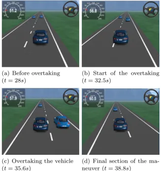
In the following a three-vehicle scenario is presented, see its illustration in Figure 4. In t= 0 the autonomous vehicle, whose reference velocity is set at 20 m/s, stops 150 m
behind the leading vehicle. Moreover, there is another vehicle coming behind with 15 m/s velocity overtakes the autonomous vehicle. Since the velocity differences the autonomous vehicle accelerates and approaches the vehicles ahead. However, it is necessary to guarantee a safe overtaking maneuver, in which the motions of both vehicles are considered. Figure 5 illustrates the different stages of the overtaking maneuver of the autonomous vehicle.
150 m
vlong(0) = 0m/s vlong(0) = 10m/s
vlong(0) = 15m/s
Fig. 4. Simulation example
(a) Before overtaking (t= 28s)
(b) Start of the overtaking (t= 32.5s)
(c) Overtaking the vehicle (t= 35.6s)
(d) Final section of the ma- neuver (t= 38.8s)
Fig. 5. Stages of the overtaking maneuver
In Figure 5(a) the motions of the vehicles in t = 28 s are illustrated. In this stage the autonomous vehicle catches up with the leading vehicle but there is the other vehicle to the left-hand-side lane, thus the velocity of the autonomous vehicle must be reduced, see the velocity profile in Figure 7(a). At t = 32.5 s the vehicle decides to start the overtaking maneuver. Thus, the autonomous vehicle is moving to the left-hand-side lane (Figure 5(b)) and the velocity is increased to perform the overtaking maneuver (Figure 6(b)).
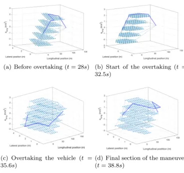
Figure 5(c) illustrates that the autonomous vehicle is to the left of the leading vehicle. However, due to the small distance from the other vehicle traveling in the same lane it is necessary to decelerate in preparation to returning to the right-hand-side lane, see the result of the decision algorithm in Figure 6(c). Finally, when a safe distance from the vehicle in the right lane is reached, the autonomous vehicle moves back to the right-hand-side lane and the reference velocity 20m/scan also be tracked, see Figure 5(d) and Figure 6(d).
(a) Before overtaking (t= 28s) (b) Start of the overtaking (t= 32.5s)
(c) Overtaking the vehicle (t = 35.6s)
(d) Final section of the maneuver (t= 38.8s)
Fig. 6. The result of the graph-based optimization Some signals of the autonomous vehicle are found in Figure 7. It can be seen that the results of the MPC controls are vlong(Figure 7(a)) andδ(Figure 7(c)), with which the safe motion of the vehicle can be guaranteed.
0 10 20 30 40 50 60
0 25 50 72 90
Time (s) vlong (km/h)
(a) Longitudinal velocityvlong
0 10 20 30 40 50 60
−1
−0.5 0 0.5 1
Time (s)
Steering angle (deg)
(b) Steering angleδ
Fig. 7. Signals of the vehicle
5. CONCLUSIONS
The paper has proposed a control strategy for the design of overtaking maneuvers in multiple vehicle scenarios.
The method is built on a probability-based approach, in which the lateral and longitudinal motions of the surrounding human-driven vehicles are predicted. The results of the prediction are incorporated in a graph-based optimal route and velocity selection algorithm. Through the algorithm the motions of the surrounding vehicles can be incorporated in the safe design of autonomous vehicle motion. The efficiency of the method has been illustrated through an overtaking simulation example with two surrounding vehicles.
REFERENCES
M. Althoff and A. Mergel. Comparison of markov chain abstrac- tion and monte carlo simulation for the safety assessment of au- tonomous cars.IEEE Transactions on Intelligent Transportation Systems, 12(4):1237–1247, Dec 2011.
K. Berntorp. Path planning and integrated collision avoidance for autonomous vehicles. In American Control Conference, pages 4023–4028, May 2017.
A. Carvalho, S. Lef´evre, G. Schildbach, J. Kong, and F. Borrelli.
Automated driving: The role of forecasts and uncertainty - A control perspective.European Journal of Control, 24:14–32, 2015.
H. Farah, S. Bekhor, A. Polus, and T. Toledo. A passing gap acceptance model for two-lane rural highways. Transportmetrica, 5(3):159–172, 2009.
J. Firl and Q. Tran. Probabilistic maneuver prediction in traffic scenarios. In Proceedings of the 5th European Conference on Mobile Robots, pages 89–94, 2011.
T. Gindele, S. Brechtel, and R. Dillmann. A probabilistic model for estimating driver behaviors and vehicle trajectories in traffic envi- ronments. In13th International IEEE Conference on Intelligent Transportation Systems, pages 1625–1631, Sept 2010.
D. Gonz´alez, J. P´erez, V. Milan´es, and F. Nashashibi. A review of motion planning techniques for automated vehicles. IEEE Transactions on Intelligent Transportation Systems, 17(4):1135–
1145, 2016.
R. Kala and K. Warwick. Motion planning of autonomous vehicles in a non-autonomous vehicle environment without speed lanes.
Engineering Applications of Artificial Intelligence, 26:1588–1601, 2013.
S. Lefevre, D. Vasquez, and C. Laugier. A survey on motion prediction and risk assessment for intelligent vehicles. Robomech Journal, 1(1):1–14, 2014.
D. Lloyd, P. Baden, D. Mais, A. Marshall, A. Bhagat, and D. Wilson.
Reported road casualties Great Britain: Annual report. Depart- ment for Transport, Sep 2016.
V. Milan´es, D. F. Llorca, J. Villagr´a, J. P´erez, C. Fern´andez, Ignacio Parra, Carlos Gonz´alez, and Miguel A.Sotelo. Intelligent automatic overtaking system using vision for vehicle detection.
Expert Systems with Applications, 39(3):3362–3373, 2012.
F. Molinari, Nguyen Ngoc Anh, and L. Del Re. Efficient mixed integer programming for autonomous overtaking. In Amer- ican Control Conference, pages 2303–2308, May 2017. doi:
10.23919/ACC.2017.7963296.
D. Moser, Z. Ramezani, D. Gagliardi, J. Zhou, and L. del Re. Risk functions oriented autonomous overtaking. In11th Asian Control Conference, pages 1017–1022, Dec 2017.
N. Murgovski and J. Sj¨oberg. Predictive cruise control with au- tonomous overtaking. In2015 54th IEEE Conference on Decision and Control (CDC), pages 644–649, Dec 2015.
N. A. Nguyen, D. Moser, P. Schrangl, L. del Re, and S. Jones.
Autonomous overtaking using stochastic model predictive control.
In11th Asian Control Conference, pages 1005–1010, Dec 2017.
K. Okamoto, K. Berntorp, and S. Di Cairano. Similarity-based vehicle-motion prediction. InAmerican Control Conference, pages 303–308, May 2017.
P. Petrov and F. Nashahibi. Modeling and nonlinear adaptive control for autonomous vehicle overtaking. IEEE Transactions on Intelligent Transportation Systems, 15(4):1643–1656, 2014.
R. Rajamani. Vehicle dynamics and control.Springer, 2005.
RoSPA. Road safety factsheet: Overtaking. The Royal Society for the Prevention of Accidents, July 2017.
J.P. Switkes, E.J. Rossetter, and J.C. Gerdes. Experimental vali- dation of the potential field lanekeeping system. Int J Automot Technol, 5(2):95–108, 2004.
J. N. Tsitsiklis. Efficient algorithms for globally optimal trajectories.
IEEE Transactions on Automatic Control, 40(9):1528–1538, Sep 1995.
D. K. Wilde. Computing clothoid segments for trajectory generation.
InIEEE/RSJ International Conference on Intelligent Robots and Systems, pages 2440–2445, Oct 2009.
C. Wissing, T. Nattermann, K. Glander, C. Hass, and T. Bertram.
Lane change prediction by combining movement and situation based probabilities. 20thIFAC World Congress, 50(1):3554 3559, 2017.
J. Xu, K. Yang, Y. Shao, and G. Lu. An Experimental Study on Lateral Acceleration of Cars in Different Environments in Sichuan, Southwest China. Discrete Dynamics in Nature and Society, page 16, 2015.