Adaptive Semi-Active Suspension Design Considering Cloud-based Road Information
Andr´as Mih´aly∗ Ad´´ am Kisari∗ P´eter G´asp´ar∗ Bal´azs N´emeth∗
∗Systems and Control Laboratory, Institute for Computer Science and Control, Hungarian Academy of Sciences,
Kende utca 13-17, 1111, Budapest, Hungary.
Abstract: Adaptive suspension control considering passenger comfort and stability of the vehicle has been researched intensively, thus several automotive companies already apply these technologies in their high-end models. Most of these systems react on the instantaneous effects of road irregularities, however, some expensive camera-based systems adapting the suspension in coherence with upcoming road conditions has already been introduced. Thereby, using oncoming road information the performance of adaptive suspension systems can be enhanced significantly.
The emerging technology of cloud computing enables several promising features for road vehicles, one of which may be the implementation of an adaptive look-ahead suspension system using historic road information gathered in the cloud database. The main novelty of the paper is the developed semi-active suspension control method in which Vehicle-to-Cloud-to-Vehicle (V2C2V) technology serves as the basis for the look-ahead road adaptation capabilities of the suspension system. The operation of the presented system is validated by a real data simulation in TruckSim simulation environment.
Keywords:Adaptive suspension, Cloud, Look-ahead, V2X, Semi-active suspension, Control 1. INTRODUCTION
Cloud technologies are considered commonplace in a wide variety of application areas. In vehicular use cases however, cloud is an untapped resource. The main motivation of our research is to exploit the advantages of cloud technologies not yet adopted by the automotive industry. Cars usu- ally have limited computational resources which can be supplemented by offloading data storage and non-realtime calculations to a cloud service, see Viereckl et al. (2014).
This practice is further encouraged by the EU regulations that oblige all new cars sold in or after 2018 to have cellular data connection embedded in them. The primary goal of the ruling is to implement an e-call service but the connection itself is universal (Schulz and Kalnina- Lukasevica (2015)). The system described in this paper operates much like the one introduced by Li et al. (2014).
The following use-case can be considered as an example: A vehicle equipped with a semi-active suspension system and our look-ahead controller is travelling along a road. The planned route is known by the controller, defined by a list of GPS coordinates. This information is transferred to a cloud service along with the current position, speed and heading via a cellular network connection. Based on this
? This work has been supported by the GINOP-2.3.2-15-2016-00002 grant of the Ministry of National Economy of Hungary and by the European Commission through the H2020 project EPIC under grant No. 739592.
The work of Bal´azs N´emeth was partially supported by the J´anos Bolyai Research Scholarship of the Hungarian Academy of Sciences and the UNKP-18-4 New National Excellence Program of the Min- istry of Human Capacities.
data the cloud application proposes a scheduling variable for the suspension of the vehicle, in advance for a specific road segment. At the same time the on-board controller calculates an other scheduling variable using real-time data of the sensors equipped on the vehicle. The two variables are combined by a decision logic and the result is fed to the suspension system. Simultaneously the vehicle collects sensor measurements regarding the current road conditions and uploads the data to the cloud service. The cloud application aggregates this information to maintain a database of road conditions.
The paper is organized as follows: in Chapter 2 we will discuss the workings and components of the whole system, including the cloud part and the suspension as well. In Chapter 3 we share the results produced in our simulation environment. Finally, in Chapter 4 conclusions are drawn.
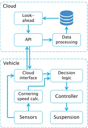
2. DESIGN OF THE SYSTEM ARCHITECTURE Our system consists of two main parts. The vehicle with the semi-active suspension system and the cloud applica- tion hosting the road information service. In this case the vehicle is simulated in TruckSim and the control algorithm runs as a Matlab script on the same computer.
The cloud application is implemented on a private infras- tructure cloud, namely MTA Cloud which is a service of the Hungarian Academy of Sciences. The application is not dependant on special features, meaning it could be hosted on other providers as well. The database engine has been chosen to be MongoDB. The decision was supported by the fact that it provides a number of features to handle
Cloud
Vehicle
Sensors Suspension Controller Cornering
speed calc.
Decision logic Cloud
interface
API Data
processing Look-
ahead
Fig. 1. System architecture
geospatial information. The Cloud application itself was written in Python. Using the Flask software framework it provides a RESTful API. The simulated vehicle connects to the cloud application using the ’webread’ function pro- vided by MATLAB.
2.1 Method of communication
The cloud application provides two functions trough the API: upload and download.
The vehicle can download a precalculated parameter from the cloud that can be used as a reference signal to configure the suspension. The properties and calculation of the parameter will be detailed later in this paper. To provide relevant information the cloud needs the planned route and current position of the vehicle. The application responds to a query by sending the parameter for a predefined distance along the path of the vehicle.
The upload functionality is meant to keep the cloud database up to date. In exchange for the advance road information a vehicle can upload its current measurements on road quality.
2.2 Data collection
The data collected in the database is always referenced by its location, hence a geospatial database is constructed. In our case a second identifier is needed to properly select data: the velocity with which the vehicle travelled at the time of the measurement. The reason for this is the fact that the deformation of the suspension is highly dependent on vehicle speed. For the calculations made by the app we need to collect the following signals:
• position (GPS coordinates)
• velocity of the vehicle
• yaw-rate of the vehicle
• horizontal, vertical and longitudinal accelerations of the vehicle body,
• vertical acceleration of the unsprung mass
The cloud application calculates the scheduling variable aforementioned for the controller when new data arrives.
This new variable is then compared with historical data for the given place and speed and then the database is updated accordingly. The comparison is necessary to filter out faulty data or intentional misinformation from the database.
2.3 Modeling and control of the semi-active adaptive suspension system
Several researchers already developed active suspension systems based on the quarter-car model with very different approaches. Although linear quadratic andH∞suspension control can guarantee good performance in both passen- ger comfort and stability, due to the fixed weighting of performances a dynamic control reconfiguration is not possible, see Zin et al. (2005). In Fergani et al. (2013) an approach using on-line road profile identification has been introduced, thus the semi-active suspension system had road adaptation capabilities.
Present paper proposes a semi-active suspension system with magnetorheological (MR) dampers discussed by sev- eral authors, see Soltane et al. (2015); Hu et al. (2017);
Chen et al. (2014). One of the main advantage of MR dampers are their practical application in suspension con- trol of road vehicles due to their quick response and low power consumption. The behavior of an MR damper can most easily be described with the Bingham model pre- sented in Sapinski and Filus (2003), where a Coulomb friction element fc is present next to the conventional shock absorber. Thus, the damping force can be expressed as:
F=fcsign( ˙q1−q˙2) +bs( ˙q1−q˙2) +f0. (1) where fc represents the frictional force, bs is the viscous damping rate and f0 is a constant force due to the accumulator.
The design is based on the commonly used two-degree-of- freedom quarter-car model shown in Figure 2.
The dynamic model of the quarter-car suspension system is written as follows:
msq¨1+bs( ˙q1−q˙2) +ks(q1−q2)+
+fcsgn( ˙q1−q˙2) +f0 = 0 muq¨2+bs( ˙q2−q˙1) +ks(q2−q1) +kt(q2−w)−
fcsgn( ˙q1−q˙2)−f0 = 0 (2) where ms is the sprung mass of the quarter vehicle, mu
represents the unsprung mass, kt is the stiffness of the tire,ks is the stiffness of the spring. Note, that q1 and q2
are the vertical displacement of the sprung mass and the unsprung mass, while road disturbance is denoted withw.
The nominal parameters of the quarter-car model for the front and rear suspension is shown in Table 1.
The goal of the design is to achieve a desired trade- off between ride comfort and road holding, while also
Fig. 2. Quarter-car model
Table 1. Quarter-car model parameters
Parameters Front Rear Unit
(symbols) suspension suspension
sprung mass (ms) 214 336 kg
unsprung mass (mu) 40 40 kg
suspension stiffness (ks) 30 60 kN/m
tire stiffness (kt) 220 220 kN/m
viscous damping (bs) 2435-5648 5235-8448 N/m/s frictional force (fc) 43.95-262.13 43.95-262.13 N
current (I) 0-0.4 0-0.4 A
taking control force into consideration. Hence, for the sake of increasing passenger comfort, the acceleration of the sprung mass must be minimized with the following optimization criterion:z1= ¨q1→0. Directional stability is guaranteed with the minimization of suspension deflection, hence z2 = (q1−q2) → 0. In order to reduce variations of side force to guarantee stability, the dynamic tire load must be minimized with the optimization criterion z3 = (q2−w) → 0. Finally, on order to avoid actuator saturation, the control force must also be considered with the optimization criterion z4 = F → 0. The measured signal is the relative displacement between the masses and the velocity of the sprung mass, i.e y= [q1−q2; ˙q1]. The control input u=F is the vertical force generated by the MR dampers.
The control of the semi-active suspension is based on the sky-hook control policy described by Yao et al. (2002), as follows:
F =
Fmax, if q˙1( ˙q1−q˙2)>0
Fmin, if q˙1( ˙q1−q˙2)<0 (3) whereFmaxis the damping force generated with the max- imal prescribed current for the MR damper (0.4A), while Fminis the minimal damping force generated without any current applied.
In order to design an adaptive semi-active suspension, the cloud-aided calculated value of scheduling variable ρ is also added to the control of the semi-active suspension.
The aim of introducing the scheduling variable ρ is to create a tunable controller, which can adapt to the road conditions and vehicle dynamics. Since selection of ρ= 0 represents the overall importance of passenger comfort and ρ= 1 stands for the road stability of the vehicle, between the edge values a mixed performance is guaranteed. The
goal of the cloud-based road roughness estimation and the on-board vehicle dynamic monitoring system is to set an appropriate value forρ, with which the suspension system adapts to the actual road conditions. The adaptation is realized by altering the current of the MR damper and the corresponding maximal damping force Fmax. Hence the parameters of the Bingham model described with (1) is altered with scheduling parameterρas follows:
Fmax = (fcmin+ρ(fcmax−fcmin))sign( ˙q1−q˙2)+
+(bmins +ρ(bmaxs −bmins ))( ˙q1−q˙2)+
+(f0min+ρ(f0max−f0min))
(4)
2.4 Data processing
The scheduling variable will be calculated in two parts. Let the first part beρ1. This variable is related to suspension deflection, which is tied to the stability of the vehicle.
ρ1 can be further divided in four parts representing the four wheels of the vehicle:ρij1 i ∈ [f =f ront, r = rear], j∈[L=lef t, R=right]
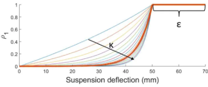
A progressive shaping function should be applied, thus the following equation is used:
ρij1 =
eκ(dmax−d −1)−
1− d
dmax−
e−κ, if d≤dmax− 1, if d > dmax−
(5)
where κis a parameter setting how progressive the func- tion should be,dis the deflection of the suspension calcu- lated as
q1ij−q2ij
and dmax is the maximal allowed sus- pension deflection calculated as max
q1ij−q2ij
. A safety margin is also present represented by to avoid reaching dmax. These parameters are considered equal for all four quarters of the vehicle.
The shaping ofρ1 is shown in Figure 3, with the red line representing the parameters used in our simulations among other possibilities.
Fig. 3. Design ofρ1
The maximum of the four values of ρij1 is selected as ρ1, thus ρ1 = max(ρij1). This way the scheduling parameter is set to a value that is always tuned towards stability, minimizing suspension and tire deflection when the sus- pension deflections would reach dangerously high values.
Otherwise the suspension can be tuned towards comfort minimizing vertical acceleration of the vehicle body.
The values calculated and stored this way can be then transmitted to the vehicle, moving along a path already
surveyed by other cars. The application interpolates be- tween such values to obtain the appropriate scheduling variable from the database considering the current speed and route plan of the vehicle.
2.5 On-board calculations
When traveling by a vehicle internet connection can not be considered reliable, therefore data caching needs to be performed. The proposed scheduling variable is down- loaded from the cloud if available, then this information is stored and used off-line to tune the suspension. The data is downloaded for a distance defined by the speed of the vehicle.
When the internet connection is active the contents of the cache can be updated when necessary. If the driver changes the planned route or simply miss an intersection the local data becomes invalid and has to be updated immediately.
The detection of such changes is carried out continuously by the on-board computer and as soon as a new route plan is available it updates accordingly. The system works just like a regular navigation software when its recalculating a route.
When there is no connection to the network the vehicle must continue to operate. In such cases the on-board software uses the contents of the cache until it runs out.
Afterward the suspension can only use the information of local sensors. This way the operation can continue without the look-ahead capability until the connection is re-established.
There is a part of the calculations that needs to be done real-time. It is important to take cornering into consider- ation. A maximal cornering speed vsaf e can be obtained regarding the danger of skidding and rollover. This cal- culation is done according to Mih´aly et al. (2014). The calculation is twofold and the next two stability parame- ters are calculated in both cases and finally a decision is made between all of them as the actual parameter to be used.
A safe velocity can be calculated for the vehicle in any curve regarding the danger of skidding as follows:
vskid= rv
ψ˙g(µ+ϕ) µ=Fo,v
Sp
ev−vskid
(6)
where v is the current velocity of the vehicle, the yaw- rate of turning is represented by ˙ψ, g is the gravitational constant, the friction is denoted by µ, and ϕ is the road superelevation. The two constants Fo,v and Sp are describing the texture of the road surface.
A safe velocity can be calculated for the vehicle in any curve regarding the danger of rollover as follows:
vroll= s v
ψ˙g 2hCOG
(b+ 2ϕhCOG) (7) here the height of the center of gravity, measured from the ground ishCOG, and bis the width of the vehicle.
Note, that the estimated maximal safe cornering velocity is chosen to be the smaller value regarding skidding or rollover, i.evsaf e= min(vskid, vroll).
When the vehicle speed approaches vsaf e the suspension should maximize safety, thusρ2is constructed as a similar progressive function asρ1, with the following equation:
ρ2=
eϑ
v vsafe−δv−1
−
1− v
vsaf e−δv
e−ϑ, if v≤vsaf e−δv 1,if v > vsaf e−δv
(8)
where δv is the safety velocity margin, ϑ is a tuning parameter defining the progressiveness of the function.
Finally, the scheduling variableρ for the suspension con- troller is selected as ρ = max(ρ1, ρ2). This way the con- troller maximizes passenger comfort when possible, but any time the cloud-based look-ahead road road informa- tion producingρ1or the real-time calculatedρ2suggests a dangerous situation the suspension of the vehicle is tuned throughρtowards safety.
3. SIMULATION RESULTS
The simulation vehicle is a compact utility truck with independent front and rear suspension and half tonne of payload. The main geometric and mass parameters of the simulated truck are shown in Table 2.
Table 2. Vehicle parameters
Parameter Value Unit
Truck mass (mt) 760 kg
Payload mass (mp) 500 kg
Distance from C.G to front axle (l1) 0.55 m Distance from C.G to rear axle (l2) 1.375 m
Track width (b) 1.26 m
Height of COG (hCOG) 0.813 m
Maximal suspension deflection (dmax) 70 mm
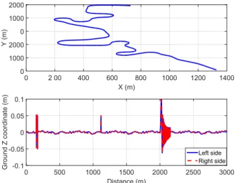
Simulation route from Gy¨ongy¨os to K´apolna has been built in TruckSim environment based on real geographical and speed limit data, see Figure 4.
Fig. 4. Real data simulation route
In order to demonstrate the effectiveness of the proposed method two different simulation has been performed and compared, one with the utility truck having passive sus- pension and another where it is equipped with the pro- posed cloud-based look-ahead semi-active suspension con- trol. Note, that only a 3 kilometre section of the route has
X (m)
0 2 00 400 600 800 1000 1200 1400
Y (m)
0 1000 2000 0 1000 2000
Distance (m)
0 500 1000 1500 2000 2500 3000
Ground Z coordinate (m) -0.1 -0.05 0 0.05 0.1
Left side Right side
Fig. 5. Geometry and roughness of the road section been considered, with the road geometry and roughness shown in Figure 5. As it can be observed in Figure 5(a), there are three major curves in the selected road section around 400 m, 1000 m and 1700 m. Moreover, there are also three different kind of road irregularities apart from the standard road roughness, as it is shown in Figure 5(b).
First, in the urban area around 100 m there is a left and right side bump following each other having 100 mm of height. This kind of road irregularity represents the effect of driving over a speed bump, which is common in urban areas. Next, after 1050 m already in the highway road section there are bumps and potholes following each other differently for the left to the right side of the lane, having a height and depth of 50 mm. This road irregularity repre- sents bad road quality with discontinuities in the asphalt.
Finally, at 2000 m there is a longitudinal sinusoidal road irregularity with growing frequency, putting extreme stress on the suspension system of the simulated vehicle. This kind of road surface is typical at bus stops, where the frequent braking of heavy road vehicles roll up the asphalt.
The speed limit is 30 km/h and 40 km/h in the urban area, which is raised to 50 km/h on the highway section.
Both simulated vehicles follow these speed limits using a conventional cruise control system (see Figure 6(a)). Note, that as shown in Figure 6(b) the yaw-rate of the simulated vehicles increase significantly in the curves, however, the laterally uneven first two bigger road irregularities also generate certain amount of yaw-rate (smaller for the vehicle with semi-active suspension).
The result of the cloud-based look-ahead road considera- tion can be observed in Figure 7(a), where the scheduling variableρis depicted. Here, the design ofρ1was evaluated with selecting = 20mm for the safety margin of the suspension, whileρ2 was designed withδv= 20km/has a safe cornering velocity margin. It is well demonstrated that as the speed limits increase, the value of ρ also increase generally with a certain amount due to bigger importance of directional stability and road holding over passenger comfort. Also, it can be observed that the in the curves (400 m, 1000 m, 1700 m)ρincreases, having bigger values (ρ ≈ 0.7) where the yaw-rate of the vehicle is bigger.
Focusing on road irregularities (100 m, 1050 m, 2000 m), the cloud-based algorithm also selects a bigger value forρ
0 500 1000 1500 2000 2500 3000
20 30 40 50 60
Distance(m)
Velocity (km/h) without control
with control
0 500 1000 1500 2000 2500 3000
−30
−20
−10 0 10 20
Distance(m)
Yawrate(deg/s) without control
with control
Fig. 6. Velocity and yaw-rate of the vehicle
on the bigger bumps, potholes and road waves, since here the aim here is to maintain the stability of the vehicle.
The actuated control forces for each quarter suspensions are depicted in Figure 7(b), having bigger values at the three main road irregularities.
The performances are compared for the two simulated vehicles. It is well demonstrated by comparing Figure 8(a) and Figure 8(b), that the amount of suspension deflection over the critical bumps have been decreased slightly for the vehicle with the proposed cloud-based look-ahead suspension control system.
Moreover, tire deformation depicted in Figure 9(a) and Figure 9(b) has been decreased significantly with the proposed method, especially at the last road irregularity (sinusoidal longitudinal waves). Thus, it has been shown that both suspension deflection and tire deformation has been improved, resulting in better stability and road holding of the vehicle. Note, that vertical acceleration connected to passenger comfort has also improved greatly over the bigger bumps (see Figure 10).
4. CONCLUSION
The paper proposed a novel cloud-based look-ahead semi- active suspension system, adapting the controller perfor- mance specifications to upcoming road conditions. The
Distance(m)
0 500 1000 1500 2000 2500 3000
ρ (-)
0 0.5 1
0 500 1000 1500 2000 2500 3000
−2000 0 2000 4000
Distance(m)
Actuated Force (N)
fL fR rL rR
Fig. 7. Scheduling variable and actuated control force
0 500 1000 1500 2000 2500 3000
−0.05 0 0.05
Distance(m)
Suspension deflection (m)
fL fR rL rR
0 500 1000 1500 2000 2500 3000
−0.05 0 0.05
Distance(m)
Suspension deflection (m)
fL fR rL rR
Fig. 8. Suspension deflection
0 500 1000 1500 2000 2500 3000
−0.06
−0.04
−0.02 0 0.02 0.04
Distance(m)
Tire deformation (m)
fL fR rL rR
0 500 1000 1500 2000 2500 3000
−0.06
−0.04
−0.02 0 0.02 0.04
Distance(m)
Tire deformation (m)
fL fR rL rR
Fig. 9. Tire deformation
0 500 1000 1500 2000 2500 3000
−10 0 10 20 30 40
Distance(m) Vertical acceleration (m/s2)
without control with control
Fig. 10. Vertical acceleration of the sprung mass
road quality information along with vehicle dynamic sig- nals had been gathered and sent to the cloud database by previous journeys of the vehicle, where it has been preprocessed to estimate the road quality and to define the corresponding scheduling variables for given road sec- tions and vehicle velocities. By this means, the vehicle is able to adapt its suspension control system in coherence with oncoming road conditions and current velocity, which improves both ride quality and stability of the vehicle. The operation of the proposed method has been demonstrated in a real data simulation in TruckSim environment.
Our results show that this look-ahead approach to a semi- active suspension control can be implemented and it can improve upon a standard passive suspension. Further tests
are required to match our system’s performance to other look-ahead type suspension systems for a fair comparison.
Other systems usually implement the look-ahead func- tionality using a camera that scans the road surface in front of and under the car. This always gives the most up-to-date information on the road conditions, but the prediction distance is very limited. The cost structure of the two systems are also radically different. The camera- based version is more costly on the vehicle hardware side and the cloud implementation needs a high availability network infrastructure what can be a big upfront cost. The differences are the most pronounced when implementing such systems at large scale. An other interesting question of our future work is the possible integration of the above mentioned two approaches to complement each other.
REFERENCES
Chen, M., Hu, Y., Li, C., and Chen, G. (2014). Semi- active suspension with semi-active inerter and semi- active damper. Proceedings of the 19th IFAC World Congress, Cape Town, South Africa, 47, 11225–11230.
Fergani, S., Menhour, L., Sename, O., Dugard, L., and D’Andr´ea-Novel, B. (2013). A new lpv/hinf semi- active suspension control strategy with performance adaptation to roll behavior based on non linear algebraic road profile estimation. 52nd IEEE Conference on Decision and Control (CDC 2013), Florence, Italy.
Hu, G., Liu, Q., Ding, R., and Li, G. (2017). Vibration con- trol of semi-active suspension system with magnetorhe- ological damper based on hyperbolic tangent model.
Advances in Mechanical Engineering, 9, 1–15.
Li, Z., Kolmanovsky, I., Atkins, E., Lu, J., Filev, D., and Michelini, J. (2014). Cloud aided semi-active sus- pension control. 2014 IEEE Symposium on Computa- tional Intelligence in Vehicles and Transportation Sys- tems (CIVTS), 76–83.
Mih´aly, A., N´emeth, B., and G´asp´ar, P. (2014). Look- ahead control of road vehicles for safety and economy purposes. European Control Conference (ECC), 714–
719.
Sapinski, B. and Filus, J. (2003). Analysis of parametric models of mr linear damper.Journal of Theoretical and Applied Mechanics, 215–240.
Schulz, M. and Kalnina-Lukasevica, Z. (2015). Regulation of the European Parliament and of the Council concern- ing type-approval requirements for the deployment of the eCall in-vehicle system based on the 112 service and amending directive 2007/46/EC. Official Journal of the European Union, L123, 77–89.
Soltane, S., Montassar, S., Mekki, O., and Fatmi, R.E.
(2015). A hysteretic bingham model for mr dampers to control cable vibrations. Journal of Mechanics of Materials and Structures, 195–206.
Viereckl, R., Assmann, J., and Raduge, C. (2014). In the fast lane - The bright future of connected cars. Booz &
Company.
Yao, G., Yap, F., Chen, G., Li, W., and Yeo, S. (2002).
Mr damper and its application for semi-active control of vehicle suspension system. Mechatronics, 963–973.
Zin, A., Sename, O., and Dugard, L. (2005). Switched hinf control strategy of automotive active suspensions.
Proceedings of the 16th IFAC world congress (WC), Praha, Czech Republic, 198–203.