Nonlinear Control of Induction Machines Using an Extended Kalman Filter

Nonlinear Control of Induction Machines Using an Extended Kalman Filter

Salima Meziane, Riad Toufouti, Hocine Benalla

Laboratory of Electrical Engineering, Constantine University Rue Bouaziz Saadi N°9

04000 Oum el Bouaghi Algeria

E-mail: [meziane_elc, toufoutidz, benalladz]@yahoo.fr

Abstract: This paper, we propose the comparative study between the performances of the proposed controller and field oriented control. With an aim of improving the field oriented control, the control of the induction motor by Input-Output linearization techniques are used to track torque and rotor flux and the scheme is extended for speed control is presented. The methods are compared in terms of their ability to handle loads on the motor shaft, their speed tracking capability and their sensitivity to operating condition variations.

To estimate the rotor flux, an open loop observer the Extended Kalman Filter (EKF) algorithm is used. A reduced dynamic motor model is used which reduces the computational requirements of the EKF. Simulation results show the effectiveness of the proposed method.

Keywords: nonlinear control, induction motors, field orientation, input output linearization, Kalman Filter

1 Introduction

Advanced control of electrical machines requires an independent control of magnetic flux and torque. For that reason it was not surprising, that the DC- machine played an important role in the early days of high performance electrical drive systems, since the magnetic flux and torque are easily controlled by the stator and rotor current, respectively.

The introduction of Field Oriented Control [1-5] meant a huge turn in the field of electrical drives, since with this type of control the robust induction machine can be controlled with a high performance. My orders have a great weakness opposite the exact knowledge of the reference mark (d, q), a low robustness against the parametric variations of the engine, and in addition with the mode of over peed where decoupling only becomes partial.

To improve the Field Oriented Control, full linearization state feedback control based on differential geometric theory [2], has been proposed in [7] for the electromagnetic torque control and in [8] for the adaptive speed control of a fifth order model of an induction motor. In this paper, a comparative study between the classical Field Oriented Control [4] and a newly proposed nonlinear controller has been carried out. The new controller is based on the theory of feedback linearization. The controller is used for the speed control of a fourth-order model of an induction motor. Since all the states are not available for direct measurement, a, open loop flux observer is proposed for the estimation of the rotor flux.

This paper is organized as follows. In Section 2, the dynamic model of the induction motor is described. The Field Oriented Control is reviewed in Section 3, and analysis of the necessity of a high performance control strategy for high speed ranges is carried on in the same section [1-5]. In Section 4, the nonlinear controller is designed for the speed and flux magnitude control of a fourth order model of an induction motor [1-8]. The observer required for the rotor flux estimation is presented in Section 5. Section 6 provides numerical simulation results, followed by the conclusion.

2 Induction Motor Modelling Using Vector Control Theory

One particular approach for the control of induction motors is the Field Oriented Control (FOC) introduced by Balaschke. Fig. 1 shows a block diagram of an indirect field-oriented control system for an induction motor [1-11]. In this system, the d-q coordinate’s reference frame is locked to the rotor flux vector rotating at the stator frequency U, as shown in Fig. 1 [2]. This result in a decoupling of the variables so that flux and torque can be separately controlled by stator direct-axis current id, and quadrature-axis current i, respectively. The stator quadrature-axis reference idsref is calculated from torque reference input Tref as [1- 5]:

Figure 1

Indirect field-oriented control

The machine equations in the stator reference frame, written in terms of space vectors, are:

dt I d R

V

s s s ^s

+ ϕ

=

(1)

r r r

r j m

dt I d

R ₊ ϕ ₋ ω ϕ

=

0 (2)

r s s

s

= L I + M I

ϕ

(3)

r r r

r

= L I + M I

ϕ

(4)

J T T dt

d − _L

Ω = (5)

) (

_{rd sq rq sd}

r

i JL i

p M

T = ϕ − ϕ

(6)

Where is the pole pair number and

r sL L

M ² 1−

σ

= ⁽⁷⁾

T rq rd

r

( ϕ , ϕ )

ϕ =

(8)

Assuming a rotor flux reference frame, and developing the previous equations with respect to the axis and axis components, leads to.

sd r rd r

rd

M i

dt d

ϕ τ τ

ϕ ₊ 1 ₌

(9)

sq rd r

JL i p M

T = ϕ

₍₁₀₎

These equations represent the basic principle of the FOC: in the rotor flux reference frame, a decoupled control of torque and rotor flux magnitude can be achieved acting on the d and q axis stator current components, respectively. A block diagram of a basic DFOC scheme is presented in Fig. 1. The rotor flux estimation is carried out by [10].

s s

s

v

s

R i

dt

d ϕ = −

(11)

)

(

s s s

r

r

L i

M

L ϕ σ

ϕ = −

(12)

The flux estimator has been considered to be ideal, being the effects due to parameter variations at low speed out of the major aim of this paper. The current controller has been implemented in the rotor flux reference frame using PI regulators with back emf compensation.

3 Technique Input-Output Linearizalion

The induction motor consists of three-phase stator windings and a rotor with short cut windings. Since the torque produced is a function of the difference between the mechanical speed and the angular speed of the supplied stator voltage, this results in a nonlinear model [1-7]. To reduce the complexity of a three-phase model, an equivalent two-phase representation is chosen. For the FOC this two- phase model is usually transformed in a rotating (d, q) reference frame [1, 3]. This allows a partial linearization of the model. This transformation is a source of problems but usually the FOC approach does not allow control the model in a stator fixed (α,β) reference frame [1]. Using nonlinear feedback allows to control the model in the stator fixed (α,β) reference frame avoiding the transformation in a rotating reference frame. The complete model in stator fixed (α,β) reference frame can is written in a linear form for a control in torque and flux:

⎪⎪

⎪

⎩

⎪⎪

⎪

⎨

⎧

⎥⎥

⎥⎥

⎦

⎤

⎢⎢

⎢⎢

⎣

⎡

+

−

⎥ =

⎦

⎢ ⎤

⎣

= ⎡

+

=

=

∑

=

2 2 1

) (

) ( 2

) ( 1

).

( )

(

β

α ϕ

ϕ

ϕ ϕ _{α β β α}

r r

s r s r r p

i

i i

I JL I

p M x

h x y h

u x g x

f x S

&

(12)

Where

⎥ ⎥

⎥ ⎥

⎥ ⎥

⎥ ⎥

⎥ ⎥

⎥

⎦

⎤

⎢ ⎢

⎢ ⎢

⎢ ⎢

⎢ ⎢

⎢ ⎢

⎢

⎣

⎡

−

−

− +

−

−

+

−

−

+ +

−

=

) 1 ( ) (

1 ) 1

(

T L s J

r I I s

r r JL p M

Tr r p r

I s Tr M

p r Tr r

I s Tr M

Tr r K K r

s p I

K r r p

Tr K I s

x f

α ϕ β

β ϕ α

ϕ β ωϕ α

β

ωϕ β ϕ α

α

ϕ β ϕ α

β ω γ

ϕ β α ω

α ϕ γ

(13)

T r

r s

s

I

I

x = [

_{α β}

ϕ

_α

ϕ

_β

Ω ]

; x =[U_sα U_sβ ]^T (14)

⎥⎥

⎥

⎦

⎤

⎢⎢

⎢

⎣

⎡

=

0 0 1 0

0

0 0 0 1 0

LS g LS

σ

σ (15)

In let us introduce the following definitions:

2 2 2 ;

1

;

Lr Ls rM R Ls Rs Lr

Ls K M Lr Ls

M Rr

Lr

Tr γ σ σ

σ = − = σ = +

= (16)

We do not develop the details of input-output linearization techniques but directly show the application on the induction motor drive [1]. The quantities which will be controlled are differentiated with respect to time until the input u appears and the derivatives of the state variables are eliminated using the state-space representation of (12) [1-9].

The derivative of dregs of a function

h ( x ) : ℜ

ⁿ

→ ℜ

along a field of vectors

[ ^{f x f}

_n

^x ]

^T

x

f ( ) =

₁

( ).... ( )

is given by:

∑

=

∂

=

ⁿ

∂

i

i i

f

f x

x x x h

h L

1

) ) ( ) (

(

₍₁₇₎

Thus the derivatives of the outputs are given by 9 For the first output

y

₁

= C

_em

u x h L x h L x h

y &

₁

= &

₁

( ) =

_{f 1}

( ) +

_{g 1}

( ).

⁽¹⁸⁾

Let us calculate

L

_f

h

₁

( x ) et L

_g

h

₁

( x )

:

)]

( )

(

) 1 )(

[(

) ) ( ) (

(

2 2 1

1 1

β α β

β α α

α β β α

ϕ ϕ ϕ

ϕ

ϕ ϕ

γ

r r s

r s r

s r s r r

r n

i

i i f

K p I I

p

I T I

L pM x x f

x x h

h L

+ Ω

+ +

Ω +

− +

−

∂ =

= ∂

•

∑

= (19)

] [

) ) ( ) (

(

1 1

1 ⁿ ϕ_rβ ϕ_rα

i

i i

g g x pK pK

x x x h

h

L = −

∂

= ∂

•

∑

=

(20)

9 For the second output

y

₁

= ϕ

_r²

)

( )

(

₂

2

2

h x L h x

y & = & =

_f ⁽²¹⁾

u x h L L x h L x h

y &&

₂

= &&

₂

( ) =

²_{f 2}

( ) +

_{g f 2}

( ).

⁽²²⁾

Let us calculate

L

_f

h

₂

( x ) , L

²_f

h

₂

( x ) et L

_g

L

_f

h

₂

( x )

:

)]

( ) (

2[ ) ) ( ) (

( ^{2 2}

1 2

2

ϕ

_rα _sα

ϕ

_rβ _sβ

ϕ

_rα

ϕ

_rβ

r n

i

i i

f M I I

x L x f

x x h

h

L = + − +

∂

= ∂

•

∑

=

(23)

) 2 (

) 2 (

) 2 )(

(6

) 2 )(

( 4 ) ) ( )(

) ( (

2 2 2

2 2

2

2 2 2 2

1

2 2

2

β α α

β β α

β β α α

β α

ϕ ϕ ϕ

ϕ

ϕ γ ϕ

ϕ ϕ

r r r s

r s r r

s r s r r r

r r r r

n

i

i i f f

T I M T I

pM

I T I

M T

M

T KM x T

x f x h x L

h L

+ +

Ω − +

+ +

−

+ +

∂ =

= ∂

•

∑

=

(24)

] 2

2 [ ) ) ( )(

) ( (

1

2

2 ⁿ _r

ϕ

_rα _r

ϕ

_rβ

i

i i f f

g

g x R K R K

x x h x L

h L

L =

∂

= ∂

• ∑

=

(25) The controller design is based on the fourth order dynamic model obtained from the (d, q) axis model of the motor under the field oriented assumptions so that either speed or flux magnitude control objective can be fulfilled [1].

The underlying design concept is to endow the closed loop system with high performance dynamics for high speed ranges while maximizing power efficiency and keeping the required stator voltage within the inverter ceiling limits [1]. In addition to filtering those control objectives, our control design aims to reduce the complexity of the control scheme, saving thereby the computation time of the control algorithm, which is an improvement over previous work found in the technical literature [1, 3]. The outputs to be controlled are the speed w and the square of the rotor flux magnitude = 4. The output vector is the sum of the relative degrees of the torque r1=1 and flux r2=2 is lower than the n=5 degree system S. we obtain a not observable dynamics of order 2.

Define the change of coordinates [11]:

Ω

=

=

=

=

=

5 4

2 3

2 2

1 1

) arctan(

) ( ) (

) (

z z

x h L z

x h z

x h z

r r f

α β

ϕ ϕ

(26)

Let us note that in the configuration where

∑

= p

i

n ri

1

p

, only the variables z1, z2, and z3 are fixed. The variables z4 and z5 are selected arbitrarily here; the followed approach is that of [1] considering z4 the rotor angle of flux.

Thus the derivatives of the outputs are given in the new coordinate system S by:

) 1 (

).

( )

( ) (

).

( )

(

5 1

5

2 1 5

4

2 2

2 3

3 2

2

1 1

1

fz T J z

z

z z p pz R z

u x h L L x h L z

z x h L z

u x h L x h L z

L r

f g f

f

g f

−

−

= +

=

+

=

=

=

+

=

&

&

&

&

&

(27)

This system can be written as:

u x h D

L h L z

z

f

f

( ).

2 2

1 2

1

+

⎥ ⎥

⎦

⎤

⎢ ⎢

⎣

= ⎡

⎥ ⎦

⎢ ⎤

⎣

⎡

&&

&

(28) Where

⎥ ⎥

⎦

⎤

⎢ ⎢

⎣

= ⎡

2

)

1

( L L h

h L x D

f g f

(29)

The decoupling matrix D(x) is singular if and only if

ϕ

_r² is zero which only occurs at the start up of the motor [11]. That is, to filtering this condition one can use in a practical setting, an open loop controller at the start up of the motor, and then switch to the nonlinear controller as soon as the flux goes up to zero. If the decoupling matrix is not singular, the nonlinear Sate feedback control is given by [1-7]:

⎥ ⎥

⎦

⎤

⎢ ⎢

⎣

⎡

+

−

+

= −

⎥ ⎦

⎢ ⎤

⎣

⎡

₋

2 2 2

1 1 1

v h L

v h L u D

u

f f s

s β α

(30) With

⎩ ⎨

⎧

=

=

2 2

1 1

y v

y v

&&

&

(31) This system can be schematized by the figure

Figure 2 Nonlinear controllers

The dynamic ones

z &

₄

et z &

₅are made not observable by the return of linearization state. From the point of view of the state and not of the input-outputs, it should then be shown that the dynamic ones of zero and stable. In let us choose the balance point of following [1-8]:

[ ^z

1

, ^z

2

, ^z

3

, ^z

4

, ^z

5

] [

^T

= 0 , ^h , 0 , ^z

4

, ^z

5

]

^T (32) The dynamics of the zeros becomes:

5

4

pz

z & =

⁽³³⁾

) 1 (

5

5

T fZ

Z & = J −

_L

−

₍₃₄₎

Where z₄ is the angle of rotor flux varying between 0 and 2π. The equation (34) and a stable first order are linear dynamics. The dynamics of zero is thus stable.

The inversion of the D(x) matrix could in theory reveal a problem bus determine it is expressed according to the model of rotor flux [1].

2 2 2

2

2 ( ) 2

2 )

det(D =− pK R_r

ϕ

_rα +

ϕ

_rβ =− pK R_r

ϕ

_r (35)

If

ϕ

_r² the matrix is no null is invertible however the mathematical description of the singularity 3^rd of starting is not problem irreversible. It is a question, indeed, of adopting a sentence of fluxing of the machine then to initialize the observer of flow, which is generally carried out. [1-5] In order to obtain a good continuation of flux and couple towards their respective reference, several strategies are possible. That given in [1-3], is to recall briefly here. The variables v1 and v2 can be calculated in the following way [1, 3]:

+ - Is, ϕ_r, Ω

+ -

D(x)

^-1

V

1

V

2

L

²f

h

1

L

²f

h

1

ϕrα ϕrβ Vsα

V_sβ

2 2

2 2 2

2 1 2

1

) (

) (

) (

rref rref

r rref

r b

b

emref emref

em a

k k

v

C C

C k v

ϕ ϕ

ϕ ϕ

ϕ _{& & &&}

&

+ +

− +

−

=

+

−

−

=

(36)

The profit Ka, Kb1 and Kb2 can be selected such as k_a +S and

2 2

1S k S

k

k_a + _b + _b are the polynomials of becoming HURWITZ not the equation of error of continuation:

⎪ ⎪

⎩

⎪ ⎪

⎨

⎧

= +

+

= +

−

=

−

=

0 0

2 2 2 1 2

1 1

2 2 2 1

e k e k e

e k e e

C C e

b b

a

emref em

rref r

&&

&

ϕ ϕ

(37)

Generally, an integral action is added in order to reject constant disturbances; as shown by Figure 3.

Figure 3 Linearized systems

Where Tref and Φref are torque and flux references. Note that the references for torque and rotor flux have to be once or twice differentiated. Thus we implement a second-order state variable filter for the flux where the states give the flux [1, 3].

Reference and their derivatives, since we want to control speed, we implement a PI controller which gives the reference for the torque Tref and compensates variations of the load torque TL. The gain kp is put on the speed measure to limit the overshoot in the speed response [1-7] (see Figure 4). For the safety of the inverter, it is advisable to limit the stator current Is of the induction motor. That keeping the torque constant while having a constant rotor flux norm results in a constant stator current. Thus, due to the decoupling of the nonlinear controller, to limit the stator current, the torque reference is limited while keeping the flux reference constant [1-8]. Torque and flux will follow the references due to the tracking capabilities of the decoupling controller.

Figure4

Speed and rotorflux-controller of input output linearization

4 Flux Observer Kalman Filter

Kalman Filter is a recursive mean squared estimator. It is capable of producing optimal estimates of system states that are not measured. The elements of the covariance matrices Q and R serve as design parameters for convergence of the system. The Kalman Filter approach assumes that the deterministic model of the motor is disturbed by centred white noise viz. the state noise and measurement noise [9]. Given the discrete Linear Time Varying (LTV) model depending on the measured speed [10].

⎩ ⎨

⎧

+

=

+ +

=

⁺

=

k k k

k k k k k k

v Cx y

w u B x A

S x

¹ ₍₃₈₎

With A, B, C expressions given in appendix

T r r s s

x

k

= [ ϕ

_α

ϕ

_β

ϕ

_α

ϕ

_β

]

_;

_u

_k

_{= [ u}

_sα

_u

_sβ

_]

^T_;

_y

_k

_{= [ i}

_sα

_i

_sβ

_]

^T ₍₃₉₎

wk and v, are mutually independent noises with covariance

. ) ( , )

( w

_k

w

^T_k

Q

_k

E v

_k

v

^T_k

R

_k

E = =

(40)

The Kalman (one step ahead) predictor minimises in a least square sense the covariance:

{ ^{( ˆ}

₁

^{) ( ˆ}

₁

⁾ }

1 − −

−

= − −

kk k T kk k k

k

E x x x x

P

(41)

And produces the optimal estimate

k T

k k k k k

T kk

T kk

k T

k k k k k

k

k T

kk T

kk k k

k k

k k

k k

k k k

Q A

P A R

C CP

C P A A

P A P

R C

CP C

P A K

x C y

K u

B x

A x

+ +

−

=

+

=

− +

+

=

−

−

−

−

−

−

−

−

− +

1 1

1

1 1

1

1 1

1 1

) (

) (

ˆ ) ˆ (

ˆ

(42)

5 Simulation Results

To validate the performances of the proposed controller, we provide a series of simulations and a comparative study between the performances of the proposed control strategy and those of the classical Field Oriented Control.

A 1.5 kW induction motor with controller is simulated using the nonlinear controller and the following motor parameters:

Vn＝230V,Lr＝0.225H，Ls＝0.225H,Lm＝0.214H, Rs＝2.89Ω，Rr＝2.39Ω，P＝2，

The controller and Kalman filter are implemented using a sampling period of 0.1 ms. In order to show the robustness of the controller with respect to variation of rotor resistance and load structure, we then have the simulation cases with desired speed controls as follows:

• The speed command is designed, but the rotor resistance is increasing 50%

during the time interval. Figure 5 shows the effects of the proposed control scheme. Obviously, the input stator voltage is increased to suppress the variation of the rotor resistance.

• The speed command is designed, but both Rr and TL, are changed. Both Rr and TL are increasing 50% during the time interval. As shown in Figure 6.

0 0.05 0.1 0.15 0.2 0.25 0.3 0.35 0.4 0.45 0.5 2.2

2.4 2.6 2.8 3 3.2 3.4 3.6

3.8 Variation of rotor resistance

Time[s]

Rr[Hom]

0 0.05 0.1 0.15 0.2 0.25 0.3 0.35 0.4 0.45 0.5 -5

-4 -3 -2 -1 0 1 2 3 4

5 Variation of torque load

Time[s]

TL[Nm]

Figure 5 Variation of rotor resistance.

Figure 6 Variation of torque load

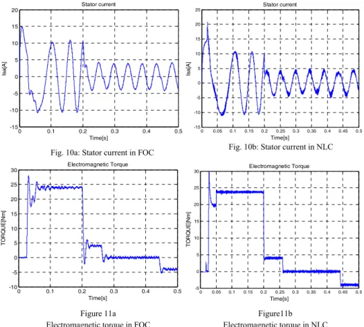
The results of simulation of proposed nonlinear controller NL_FOC and shift classical Field Oriented Control FOC of induction motor is shown in the figures (7 to 16) respectively. In the first case where one considers only one variation of torque load TL shown in the figures (7a, 8a, 9a and 11a), results of simulation the time histories of speed, flux magnitude tracking and current behavior are reported on the figures (7 to 10), for of the Field oriented Control (FOC) and nonlinear controller (NLC) on the figures (7b, 8b, 9b and 11b). As the figures show, it is observed that the speed tracks the reference values adequately well, for two methods. That is, with load torque perturbation. Figure 7a, show the flux presented the ripple around that for reference in FOC method, but the response of the flux are very good in NLC, we can observe an optimal reduction of the electromagnetic torque distortion, as shown in Figure 11b. It also appears that the rotor speed fits to the speed reference trajectory. The applied load torque has no effect on the flux and its effect on the speed is rapidly compensated. In the second test of simulation we make the resistances variations (Rr and TL).

The simulation results on the figures (12-16) shows that a good tracking performance is achieved and the above results demonstrate that the proposed controller has strong robustness properties in the presence of load disturbance and parameter variations. Consequently, the use of the proposed feedback nonlinear control scheme can solve the control problem of induction machines in the presence of uncertainties in load torque and resistance parameters variations without rotor resistance estimation.

5.1 Variations of Load Torque

Figure 7a Magnitude of rotor flux in FOC

Figure 7b

Magnitude of rotor flux in NLC

Figure 8a Rotor speed in FOC

Figure 8b Rotor speed in NLC

Figure 9a

Error between reference and Rotor speed in FOC

Figure 9b

Error between reference and Rotor speed in NLC

0 0.1 0.2 0.3 0.4 0.5

0 0.2 0.4 0.6 0.8 1 1.2

1.4 Reference Rotor flux and Rotor flux

Time[s]

phir[Wb] and phiref[Wb]

phir phiref

0 0.1 0.2 0.3 0.4 0.5

-10 0 10 20 30 40 50 60 70

80 Rotor Speed and Reference Rotor Speed

Time[s]

Wref [Rad/S] and Wr[Rad/S]

Wr Wref

0 0.05 0.1 0.15 0.2 0.25 0.3 0.35 0.4 0.45 0.5 -2

-1.5 -1 -0.5 0 0.5 1 1.5

2 Error between reference and Rotor speed

Time[s]

Error speed[Rad/S]

0 0.05 0.1 0.15 0.2 0.25 0.3 0.35 0.4 0.45 0.5

0 0.2 0.4 0.6 0.8 1 1.2

1.4 Reference Rotor flux and Rotor flux

Time[s]

phir[Wb] and phiref[Wb]

phir phiref

0 0.05 0.1 0.15 0.2 0.25 0.3 0.35 0.4 0.45 0.5 0

10 20 30 40 50 60 70

80 Rotor Speed and Reference Rotor Speed

Time[s]

Wref [Rad/S] and Wr[Rad/S]

Wr Wref

0 0.05 0.1 0.15 0.2 0.25 0.3 0.35 0.4 0.45 0.5

-2 -1.5 -1 -0.5 0 0.5 1 1.5

2 Error between reference and Rotor speed

Time[s]

Error speed[Rad/S]

Figure 11a Electromagnetic torque in FOC

Figure11b

Electromagnetic torque in NLC Fig. 10a: Stator current in FOC

0 0.1 0.2 0.3 0.4 0.5

-15 -10 -5 0 5 10 15

20 Stator current

Time[s]

Isa[A]

0 0.1 0.2 0.3 0.4 0.5

-10 -5 0 5 10 15 20 25

30 Electromagnetic Torque

Time[s]

TORQUE[Nm]

Fig. 10b: Stator current in NLC

0 0.05 0.1 0.15 0.2 0.25 0.3 0.35 0.4 0.45 0.5 -15

-10 -5 0 5 10 15 20

25 Stator current

Time[s]

Isa[A]

0 0.05 0.1 0.15 0.2 0.25 0.3 0.35 0.4 0.45 0.5 -5

0 5 10 15 20 25

30 Electromagnetic Torque

Time[s]

TORQUE[Nm]

Figure 12a Magnitude of rotor flux in FOC

0 0.1 0.2 0.3 0.4 0.5

0 0.2 0.4 0.6 0.8 1 1.2

1.4 Reference Rotor flux and Rotor flux

Time[s]

phir[Wb] and phiref[Wb]

phir phiref

Figure 12b Magnitude of rotor flux in nlC

0 0.05 0.1 0.15 0.2 0.25 0.3 0.35 0.4 0.45 0.5 0

0.2 0.4 0.6 0.8 1 1.2

1.4 Reference Rotor flux and Rotor flux

Time[s]

phir[Wb] and phiref[Wb]

phir phiref

5.2 Variations of Rotor Resistance and Torque Load

Fig. 13a: Rotor speed in FOC

0 0.1 0.2 0.3 0.4 0.5

0 10 20 30 40 50 60 70

80 Rotor Speed and Reference Rotor Speed

Time[s]

Wref [Rad/S] and Wr[Rad/S] Wr

Wref

Fig. 14a: Error between reference and Rotor speed inFOC

0 0.05 0.1 0.15 0.2 0.25 0.3 0.35 0.4 0.45 0.5 -2

-1.5 -1 -0.5 0 0.5 1 1.5 2

Error between reference and Rotor speed

Time[s]

Error speed[Rad/S]

Fig. 15a: Stator current in FOC

0 0.1 0.2 0.3 0.4 0.5

-15 -10 -5 0 5 10 15

20 Stator current

Time[s]

Isa[A]

0 0.1 0.2 0.3 0.4 0.5

-10 -5 0 5 10 15 20 25

30 Electromagnetic Torque

Time[s]

TORQUE[Nm]

Fig. 16a: Electromagnetic torque in FOC

Fig. 13b: Rotor speed in NLC

0 0.05 0.1 0.15 0.2 0.25 0.3 0.35 0.4 0.45 0.5

0 10 20 30 40 50 60 70

80 Rotor Speed and Reference Rotor Speed

Time[s]

Wref [Rad/S] and Wr[Rad/S]

Wr Wref

Fig. 14b: Error between reference and Rotor speed inNLC

0 0.05 0.1 0.15 0.2 0.25 0.3 0.35 0.4 0.45 0.5

-2 -1.5 -1 -0.5 0 0.5 1 1.5

2 Error between reference and Rotor speed

Time[s]

Error speed[Rad/S]

Fig. 15b: Stator current in NLC

0 0.05 0.1 0.15 0.2 0.25 0.3 0.35 0.4 0.45 0.5

-15 -10 -5 0 5 10 15 20

25 Stator current

Time[s]

Isa[A]

0 0.05 0.1 0.15 0.2 0.25 0.3 0.35 0.4 0.45 0.5 -10

-5 0 5 10 15 20 25

30 Electromagnetic Torque

Time[s]

TORQUE[Nm]

Conclusion

In this paper, two control techniques have been compared for induction motors':

classical Field Oriented control, and input-output linearization control, proposed by the current authors. From the comparative study, one can conclude that the two methods demonstrate nearly the same dynamic behaviour. However, the input- output linearization controller shows better performance than the Field Oriented controller in speed tracking at high speed ranges. The numerical simulations validate the performances of the proposed method and even in the unknown parameter case and achieve better speed and rotor flux tracking.

References

[1] Marino, R., Peresada, S., Valigi, P., Adaptive Input-Output Linearizing Control of Induction Motors, IEEE Automat. Contr., Vol. 38, No. 2, Feb.

1993, pp. 208-221

[2] A. Merabet, M Ouhrouche, R. T. Bui, H. Ezzaidi, Nonlinear PID Predictive Control of Induction Motor Drives, IFAC Workshop on NMPC for Fast Systems. October 9-11, 2006, Grenoble, France

[3] Raumer, T., von., J., Dion, M., and Dugard, L., Adaptive Nonlinear Speed and Torque Control of Induction Motors, in Proc. European Contr. Conf., Groningen, Netherlands, 1993

[4] Fekih, A., Fahmida, N., Chowdhury, On Nonlinear Control of Induction Motors: Comparison of two Approaches, Proceeding of the 2004 American Control Conference Boston, Massachusetts, June 30-July 2, 2004

[5] Hou, Lee., Ban, Li., Chen, Fu., Nonlinear Control of Induction Motor with Unknown Rotor Resistance and Load Adaptation, Proceedings of the American Control Conference Arlington, VA 2001, June 25-27

[6] Thomas Von Raumer., J., Dion, M., and Dugard, Luc, Thomas, Jean Luc.:

Applied Nonlinear Control of an Induction Motor Using Digital Signal Processing, IEEE Transactions On Control Systems Technology, December 1994,Vol. 2, No. 4

[7] Fekih, A., Ennaceur, Benhadj Braiek, Design of a Multimodel Approach for Nonlinear Control of Induction Motor Drives, Proceedings of the IEEE SMC 2002, TP 1I7

[8] Thomas Von Raumer., Dion, Jean Michel. and Dugard, Luc., Adaptive Nonlinear Control Of Induction Motors With Flux Observer, The authors are also with the GDR CNRS Autometique

[9] Ramdane, H., Redouane, T., Boucher, P., Dumur, D. , End Point Constraints Nonlinear Predictive Control with Integral Action for Induction Motor, Proceedings of the 2004 IEEE International Conference on Control Applications Taipei, Taiwan, September 2-4, 2004

[10] Thongam, J. S., Ouhrouche, M., Beguenane, R., Sensorless Indirect Vector Control of Induction Motor Drive Robust Against Rotor Resistance Variation, Proceeding of Power and Energy Systems, 2004, p. 448

[11] Maaziz, M. K., Boucher, P., Dumur, D., Flux and Speed Tracking of an Induction Motor Based on Nonlinear Predictive Control and Feedback Linearization, Proceedings of the American Control Conference San Diego, California, June 1999