Indirect Rotor Field-oriented Control (IRFOC) of a Dual Star Induction Machine (DSIM) Using a Fuzzy Controller
Radhwane Sadouni, Abdelkader Meroufel
Intelligent Control and Electrical Power Systems Laboratory (ICEPS) Djillali Liabes University, BP 89 Sidi Bel-Abbes, Algeria
redouanesadouni@gmail.com; ameroufel@yahoo.fr
Abstract: We present in this paper, a comparative study between a PI regulator and fuzzy regulator for a control speed of a Dual Star Induction Machine (DSIM) supplied with a two PWM voltage source inverter (VSI) and decoupled by field-oriented control (FOC).The simulation results illustrate the robustness and efficiency of the fuzzy regulator to the parametric variations.
Keywords: dual star induction machine (DSIM); field-oriented control (FOC); fuzzy logic
1 Introduction
In industrial applications in which high reliability is demanded, a multi-phase induction machine instead of traditional three-phase induction machine is used.
The advantages of multi-phase drive systems over conventional three-phase drives are: the total rating of system is multiplied, the torque pulsations will be smoothed, the rotor harmonic losses as well as the harmonics content of the DC link current will be reduced. And the loss of one machine phase does not prevent the machine working, thus improving the system reliability [1].
A common type of multiphase machine is the dual star induction machine (DSIM), also known as the six phase induction machine. These machines have been used in many applications (pumps, fans, compressors, rolling mills, cement mills, mine hoists …[2]) due to their advantages in power segmentation, reliability, and minimized torque pulsations. Such segmented structures are very attractive for high-power applications since they allow the use of lower rating power electronic devices at a switching frequency higher than the one usually used in three-phase AC machine drives [3].
The main difficulty in the asynchronous machine control resides in the fact that complex coupling exists between the field and the torque. The space vector control assures decoupling between these variables, and the torque is made similar to that of a DC machine [4].
In Field-oriented Control (FOC), three types of orientation exist: rotor field orientation, stator field orientation and rotating field orientation. In this paper, the rotor field-oriented control is applied to the DSIM using PI and fuzzy regulators.
2 Machine Model
A schematic of the stator and rotor windings for a machine dual three phase is given in Fig. 1. The six stator phases are divided into two wyes-connected three- phase sets labeled As1, Bs1, Cs1 and As2, Bs2, Cs2 whose magnetic axes are displaced by an angle α=30°. The windings of each three-phase set are uniformly distributed and have axes that are displaced 120° apart. The three-phase rotor windings Ar, Br, Cr are also sinusoidally distributed and have axes that are displaced apart by 120°
[5].
The following assumptions are made: [4], [6]:
- Motor windings are sinusoidally distributed;
- The two stars have the same parameters;
- The magnetic saturation, the mutual leakage inductances and the core losses are negligible;
- Flux path is linear.
Figure 1
Windings of the dual star induction machine Bs1
Cr
Br
Cs2
α θ
As1
As2
Ar
Cs1 Bs2
The voltage equations of the dual star induction machine are as follow [7] [8]:
[ ] [ ][ ] [ ]
[ ] [ ][ ]
[ ] [ ][ ]
r r[ ]
r rcrb ra
s2 s2
s2 sc2 sb2 sa2
s2
s1 s1
s1 sc1 sb1 sa1
s1
dt I d R V V V 0
dt I d R V
V V V
dt I d R V V V V
Φ +
=
⎥⎥
⎥
⎦
⎤
⎢⎢
⎢
⎣
⎡
=
⎥⎦
⎢ ⎤
⎣
⎡Φ +
=
⎥⎥
⎥
⎦
⎤
⎢⎢
⎢
⎣
⎡
=
Φ +
=
⎥⎥
⎥
⎦
⎤
⎢⎢
⎢
⎣
⎡
=
(1)
Where:
Rsa1 = Rsb1 = Rsc1 = Rs1 : Stator resistance 1.
Rsa2 = Rsb2 = Rsc2 = Rs2 : Stator resistance 2.
Rra = Rrb = Rrc = Rr : Rotor resistance.
[ ] [ ] [ ]
⎥⎥
⎥
⎦
⎤
⎢⎢
⎢
⎣
⎡
=
⎥⎥
⎥
⎦
⎤
⎢⎢
⎢
⎣
⎡
=
⎥⎥
⎥
⎦
⎤
⎢⎢
⎢
⎣
⎡
=
r r r
r s2 s2 s2
s2 s1 s1 s1
s1
R 0 0
0 R 0
0 0 R R
; R 0 0
0 R 0
0 0 R R
; R 0 0
0 R 0
0 0 R R
(2)
[ ] [ ] [ ]
⎥⎥
⎥
⎦
⎤
⎢⎢
⎢
⎣
⎡
=
⎥⎥
⎥
⎦
⎤
⎢⎢
⎢
⎣
⎡
=
⎥⎥
⎥
⎦
⎤
⎢⎢
⎢
⎣
⎡
=
rc rb ra
r sc2 sb2 sa2
s2 sc1 sb1 sa1
s1
I I I I ; I I I I
; I I I I
(3)
[ ] [ ] [ ]
Φ Φ Φ ;
Φ Φ Φ
; Φ Φ Φ
rc rb ra
r sc2 sb2 sa2
s2 sc1 sb1 sa1
s1
⎥⎥
⎥
⎦
⎤
⎢⎢
⎢
⎣
⎡
= Φ
⎥⎥
⎥
⎦
⎤
⎢⎢
⎢
⎣
⎡
= Φ
⎥⎥
⎥
⎦
⎤
⎢⎢
⎢
⎣
⎡
= Φ
(4)
The expressions for stator and rotor flux are [7]:
⎥⎥
⎥
⎦
⎤
⎢⎢
⎢
⎣
⎡
⎥⎥
⎥
⎦
⎤
⎢⎢
⎢
⎣
⎡
=
⎥⎥
⎥
⎦
⎤
⎢⎢
⎢
⎣
⎡
] [I
] [I
] [I . ] [L ] [L ] [L
] [L ] [L ] [L
] [L ] [L ] [L ]
[Φ ] [Φ
] [Φ
r s2 s1
rr rs2
rs1
s2r s2s2
s2s1
s1r s1s2
s1s1
r s2 s1
(5)
Where:
[Ls1s1] : Inductance matrix of the star 1.
[Ls2s2] : Inductance matrix of the star 2.
[Lrr] : Inductance matrix of the rotor.
[Ls1s2]: Mutual inductance matrix between star 1 and star 2.
[Ls2s1]: Mutual inductance matrix between star 2 and star 1.
[Ls1r] : Mutual inductance matrix between star 1 and rotor.
[Ls2r] : Mutual inductance matrix between star 2 and rotor.
[Lrs1] : Mutual inductance matrix between rotor and star 1.
[Lrs2] : Mutual inductance matrix between rotor and star 2.
The expression of the electromagnetic torque is then as follows [7] [9] [10]:
[ ] [ ][ ] [ ] [ ][ ]
⎟⎠
⎜ ⎞
⎝
⎛ +
⎟⎠
⎜ ⎞
⎝
=⎛ s1 s1r r s2 Ls2r Ir
dθ I d I . dθ L I d 2 . p Tem
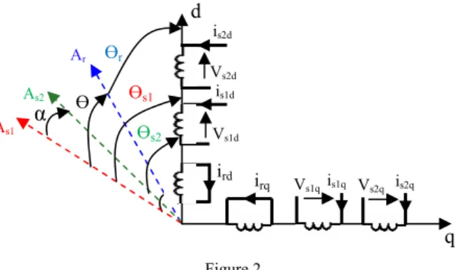
(6) The Park model of the dual star induction machine in the references frame at the rotating field (d, q) is defined by the following equations system (7) [11].
Figure 2 represents the model of the DSIM in the Park frame.
rd rq sr
rq r
rq sr rd rd
r
s2d s s2q s2q
s2 s2q
s2q s s2d s2d
s2 s2d
s1d s s1q s1q
s1 s1q
s1q s s1d s1d
s1 s1d
Φ dt ω
dΦ I
R 0
Φ dt ω
dΦ I
R 0
Φ ω dt Φ
I d R V
Φ ω dt Φ
I d R V
Φ ω dt Φ
I d R V
Φ ω - dt Φ
I d R V
+ +
=
− +
=
+ +
=
− +
=
+ +
=
+
=
(7)
Figure 2
Representation of DSlM in the Park frame
q
As1
As2
Ar
Vs2d
Vs1d
ird irq Vs1q is1q Vs2q is2q
is1d
is2d
d
α
Өr
Ө Өs1
Өs2
Where:
) I I (I L I L
) I I (I L I L
) I I (I L I L
) I I (I L I L
) I I (I L I L
) I I (I L I L
rq s2q s1q m rq r rq
rd s2d m s1d
rd r rd
rq s2q m s1q
s2q s2 s2q
rd s2d m s1d
s2d s2 s2d
rq s2q m s1q
s1q s1 s1q
rd s2d m s1d
s1d s1 s1d
+ + +
= Φ
+ + +
= Φ
+ + +
= Φ
+ + +
= Φ
+ + +
= Φ
+ + +
= Φ
(8)
Lm: Cyclic mutual inductance between stator 1, stator 2 and rotor.
The mechanical equation is given by [8]:
dt T T F Ω
dΩ
J = em − r − r
(9)
With :
[
(I I )- (I I )]
L L p L
T rd s1q s2q rq s1d s2d
m r
m
em Φ + Φ +
= +
(10)
3 Voltage Source Inverter Modelling
The voltage source inverter (VSI) is a static converter constituted by switching cells generally with transistors or thyristors GTO for high powers (Figure 3). The operating principle can be expressed by imposing on the machine the voltages with variable amplitude and frequency starting from a standard network 220/380 V – 50 Hz [12].Voltages at load neutral point can be given by the following expression [13]:
⎥⎥
⎥
⎦
⎤
⎢⎢
⎢
⎣
⎡
⎥⎥
⎥
⎦
⎤
⎢⎢
⎢
⎣
⎡
−
−
−
−
−
−
=
⎥⎥
⎥
⎦
⎤
⎢⎢
⎢
⎣
⎡
13 12 11
K K K 2 1 1
1 2 1
1 1 2 3 E V
V V
an an an
(11)
This modelling for the two converters that feed the DSIM.
4 Field-oriented Control
The objective of space vector control is to assimilate the operating mode of the asynchronous machine at the one of a DC machine with separated excitation, by decoupling the torque and the flux control. The IRFOC consists in makingΦqr=0 while the rotor direct flux Φdrconverges to the reference Φr* [4] [14].
By applying this principle (Φqr=0 and Φdr =Φr*) to equations (7) (8) and (10), the finals expressions of the electromagnetic torque and slip speed are:
) I L (I
L p L
T r s1q s2q
r m
m em
∗
∗
∗ +
+ Φ
=
(12)
(
L R LL)
(I I )w s1q s2q
r m r
r m ∗ ∗
∗
∗ +
Φ
= +
sr
(13) The stators voltage equations are:
) I
(L ω dtI L d I R V
) w T I (L ω dtI L d I R V
) I
(L ω dtI
L d I R V
) w T I L ( ω dtI L d I R V
s2d r s2 s s2q s2 s2q s2 s2q
r r s2q s2 s s2d s2 s2d s2 s2d
s1d r s1 s s1q s1 s1q s1 s1q
r r s1q s1 s s1d s1 s1d s1 s1d
∗ ∗
∗
∗
∗ ∗
∗
∗ ∗
∗
∗
∗ ∗
∗
Φ + +
+
=
Φ +
− +
=
Φ + +
+
=
Φ +
− +
=
sr sr
(14)
The torque expression shows that the reference fluxes and stator currents in quadrate are not perfectly independent. Thus, it is necessary to decouple the torque and flux control of this machine by introducing new variables:
K11 K12 K13
E n
T11 T12 T13
D11 D12 D13
T22
T21 T23
D21 D22 D23
o
ia ib ic a
b
c
Van Vbn Vcn
VT1 VT2 VT3
E 2
E 2
Figure 3
Voltage Source Inverter scheme
s2q s2
s2q s2 s2q
s2d s2
s2d s2 s2d
s1q s1
s1q s1 s1q
s1d s1
s1d s1 s1d
dt I L d I
R V
dt I L d I
R V
dt I L d I
R V
dt I L d I
R V
+
=
+
=
+
=
+
=
(15)
The equation system (15) shows that the stator voltages (Vs1d, Vs1q, Vs2d, Vs2q) are directly related to the stator currents (Is1d, Is1q, Is2d, Is2q). To compensate the error introduced at decoupling time, the voltage references (Vs1d*, Vs2d*, Vs1q*, Vs2q*) at constant fluxare given by:
s2qc s2q
s2q
s2dc s2d
s2d
s1qc s1q
s1q
s1dc s1d
s1d
V V
V
V V
V
V V
V
V V
V
+
=
−
=
+
=
−
=
∗
∗
∗
∗
(16)
With:
) r I
(L ω V
) w T
I (L ω V
) I
(L ω V
) w T
I L ( ω V
s2d s2 s s2qc
r r s2q s2 s s2dc
r s1d s1 s s1qc
r r s1q s1 s s1dc
∗
∗
∗
∗ ∗
∗ ∗
∗
∗ ∗
Φ +
=
Φ +
=
Φ +
=
Φ +
=
sr sr
(17)
For a perfect decoupling, we add stator current regulation loops (Is1d, Is1q, Is2d, Is2q) and we obtain at their output stator voltages (Vs1d, Vs1q, Vs2d, Vs2q).The decoupling bloc scheme in voltage (Field-oriented control FOC) is given in Figure 4.
5 Indirect Method Speed Regulation
The principle of this method consists in not using rotor flux magnitude but simply its position calculated with reference sizes. This method eliminates the need to use a field sensor, but only the one of the rotor speed [15].
The speed regulation scheme by IFOC of the DSIM is given in Figure 5.
Figure 4 Decoupling bloc in voltage Tem*
isa1
isb1
isc1 P a r k
is2q
Φr* is1d*
-
vs1d*
is2d
vs2q*
is1d
is1q
vs2d*
vs1q*
(θs*-α) θs* +
÷
Ls2
÷
Ls1
Ls2 Rr
is1q*
ωs
ωsr
ωr
ωm +
- +
+
+
+ -
+ +
+ -
+ +
- +
+
+ +
+ + Ls1
- + Lr
Rr+(Lr+Lm)s
2RrLm
(Lr+Lm) 2pLm
PI
PI
PI
PI (Lr+Lm)
2pLm +
P a r k
∫
∫
p
+
isa2
isb2
isc2
Figure 5
Indirect method speed regulation E
isa1
ωm
Φr* ωs*
vs2d* vs2q* vs1q* vs1d*
θsref
isb1 isc1
isa2 isb2 isc2 θsref -α PWM_VSI_2 Field Weakening
p
PWM_VSI_1 Park-1
θsref vsa1* vsb1* vsc1*
Park-1 vsc2* vsb2 * Tem*
DSIM
PI
E F
O
C
∫
ω*
+ _
vsa2*
5.1 Robustness Tests
The robustness of the indirect method speed regulation of the DSIM is visualized for two tests: the first is the varying of rotor resistance Rr (Rr = 2Rrn at t =1 s); the second increasing of inertia J (J =2Jn at t =1 s).
5.2 Results and Discussion
0 1 2 3 4
0 100 200 300 400
Temps (s)
Vitesse (rad/s)
0 1 2 3 4
-20 0 20 40 60
Temps (s)
Couple (N.m)
0 1 2 3 4
-1 0 1 2
Temps (s)
Flux rotoriques(Wb)
0 1 2 3 4
-10 0 10 20
Temps (s)
Courants statoriques(A)
phird phirq
isd1 isq1
Figure 6
Indirect method speed regulation with load torque Tr = 14 N.m between [1.5 2.5] s
Speed (rad/s) Rotor filed (Wb) Torque (N.m)Stators currents (A)
Time (s) Time (s)
Time (s) Time (s)
0 1 2 3 4
0 100 200 300 400
Temps (s)
Vitesse (rad/s)
0 1 2 3 4
-20 0 20 40 60
Temps (s)
Couple (N.m)
0 1 2 3 4
-1 0 1 2
Temps (s)
Flux rotoriques(Wb)
0 1 2 3 4
-10 0 10 20
Temps (s)
Courants statoriques(A)
isd1isq1 phirq
phird
Figure 7
DSIM Comportment with rotor resistance variation (R = 2Rn at t = 1 s)
Speed (rad/s) Rotor filed (Wb) Torque (N.m)Stators currents (A)
Time (s) Time (s)
Time (s) Time (s)
The speed reaches its reference value (300 rad/s) after (0.78 s) with an overtaking of (0.32%) of the reference speed (Figure 6). The perturbation reject is achieved at (0.1 s). The electromagnetic torque compensates the load torque and reaches at starting (60 N.m).
Simulation results show the regulation sensibility with PI for rotor resistance variation. We note that the decoupling is affected. The inertia variation increases the inversion time of rotating direction (Figures 7 and 8).
6 Fuzzy Logic Principle
The fuzzy logic control (FLC) has been an active research topic in automation and control theory since Mamdani proposed in 1974 based on the fuzzy sets theory of Zadeh (1965) to deal with the system control problems that are not to model [16].
The structure of a complete fuzzy control system is composed of the following blocs: Fuzzification, Knowledge base, Inference engine, Defuzzification. Figure 9 shows the structure of a fuzzy controller [16].
The Fuzzification module converts the crisp values of the control inputs into fuzzy values. A fuzzy variable has values which are defined by linguistic variables (fuzzy sets or subsets) such as: low, medium, high, big, slow . . . where each is defined by a gradually varying membership function. In fuzzy set terminology, all the possible values that a variable can assume are named the universe of discourse, and the fuzzy sets (characterized by membership function) cover the whole universe of discourse. The membership functions can be triangular, trapezoidal … [16].
0 1 2 3 4 5
-100 -50 0 50 100
Temps (s)
Couple (N.m)
0 1 2 3 4 5
-1 0 1 2
Temps (s)
Flux rotoriques(Wb)
0 1 2 3 4 5
-400 -200 0 200 400
Temps (s)
Vitesse (rad/s)
0 1 2 3 4 5
-20 0 20 40
Temps (s)
Courants statoriques(A)
phirq
phird isq1
isd1
Figure 8
DSIM Comportment with inertia variation (J=2Jn at t=1 s)
Speed (rad/s) Rotor filed (Wb) Stators currents (A)Torque (N.m)
Time (s) Time (s)
Time (s) Time (s)
Figure 10
Fuzzyfication with five membership functions
0.5
-1 -0.5 0 0.5 1
PL
NL NS ZE PS
0 1
Figure 9 Fuzzy controller structure
FLC X* Error
+ _ d dt
Defuzzification u Data Base
Inference Fuzzification
The number of linguistic value (small negative, middle negative, positive...), represented by the membership functions can vary (for example three, five or seven). An example of Fuzzyfication is illustrated in (Figure 10) for a single variable of x with triangular membership function; the corresponding linguistic values are characterized by the symbols likewise:
NL: Negative Large.
NS: Negative Small.
ZE: Zero Equal.
PS: Positive Small.
PL: Positive Large.
A fuzzy control essentially embeds the intuition and experience of a human operator, and sometimes those of a designer and researcher. The data base and the rules form the knowledge base which is used to obtain the inference relation. The data base contains a description of input and output variables using fuzzy sets. The rule base is essentially the control strategy of the system. It is usually obtained from expert knowledge or heuristics; it contains a collection of fuzzy conditional
statements expressed as a set of If-Then rules [16]. An example of a rule type: if x1 is positive large, x2 is zero equal, then, u is positive small, where: x1 and x2 represent two input variables of the regulator likewise: the gap of variable to regulate and its variation, and u represent the control variable (output).
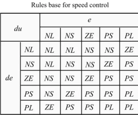
Table 1 presents a two linguistic variables of input; the speed error « e »and its variation « de »and the output variable « du ».
The mathematical procedure of converting fuzzy values into crisp values is known as ’Defuzzification’. A number of Defuzzification methods have been suggested.
The choice of Defuzzification methods usually depends on the application and the available processing power. This operation can be performed by several methods of which center of gravity (or centroid) and height methods are common [16].
7 Speed Control by Fuzzy Regulator
The principle of the fuzzy speed control is the same one as that given in Figure 5, but we have changed the classical PI speed controller with a fuzzy logic controller (FLC); the other current regulators remain of classical type. The principle scheme of the speed regulation by fuzzy logic is given in Figure 11.
7.1 Results and Discussion
The speed reaches its reference value after (0.43 s) without overtaking. The electromagnetic torque compensates the load torque and presents at starting a value equal to (80 N.m) (Figure 12).
Table 1 Rules base for speed control
du NL
e
ZE PS PL NS
NL NS ZE PS PL
NL NL NS NS
ZE PS PS PL PL PL PS PS NL NS NS ZE NS NS ZE NS ZE PS ZE PS PS de
The simulation results show the insensitivity of fuzzy control to machine parameters variation (Increasing of Rr and J of 100% of theirs nominal value) (Figure 13, and Figure 14). The inversion time of the speed is without overtaking, with a negative torque equal to (45 N.m) (Figure 14). Direct rotor field (Φdr) follows the reference value (1 Wb) and the quadrature component (Φqr) is null.
Figure 11
Indirect method fuzzy speed regulation E
isa1
ωm
Φr* ωs*
vs2d* vs2q* vs1q* vs1d*
θsref
isb1 isc1
isa2 isb2 isc2 θsref -α PWM_VSI_2 Field Weakening
p
PWM_VSI_1 Park-1
θsref vsa1* vsb1* vsc1*
Park-1 vsc2* vsb2 * Tem*
DSIM
E F
O
C
∫
ω*
+ _
vsa2* FLC
T(N)
0 1 2 3 4
-200 0 200 400
Temps (s)
Vitesse (rad/s)
0 1 2 3 4
-50 0 50 100
Temps (s)
Couple (N.m)
0 1 2 3 4
-1 0 1 2
Temps (s)
Flux rotoriques (Wb)
0 1 2 3 4
-10 0 10 20
Temps (s)
Courants statoriques (A)
isd1isq1 phirq
phird
Figure 12
Speed regulation using fuzzy regulator, with applying resistant torque (Tr =14 N.m) between [1.5 2.5] s Time (s)
Time (s)
Time (s) Time (s)
Speed (rad/s)Rotor filed (Wb) Torque (N.m)Stators currents (A)
Conclusions
In this paper we are presented a Field-oriented Control (FOC) of a Dual Star Induction Machine (DSIM). Two types of regulator are tested for the machine speed regulation: a PI regulator and a fuzzy regulator. The simulation results show the sensitivity of PI regulators to the parameters variation of the DSIM. The fuzzy regulator has very good dynamic performances compared with the conventional PI regulator: (a small response time, overtaking negligible, a small speed inversion time). Additionally, the robustness tests show that the fuzzy regulator is
0 1 2 3 4
-50 0 50 100
Temps (s)
Couple (N.m)
0 1 2 3 4
-1 0 1 2
Temps (s)
Flux rotoriques(Wb)
0 1 2 3 4
-20 -10 0 10 20
Temps (s)
Courants statoriques(A)
0 1 2 3 4
-400 -200 0 200 400
Temps (s)
Vitesse (rad/s)
isd1isq1 phirq
phird
Figure 14
DSIM Comportment with inertia variation (J=2Jn at t=1 s) Time (s) Time (s)
Time (s) Time (s)
Torque (N.m)
Speed (rad/s) Rotor filed (Wb) Stators currents (A)
0 1 2 3 4
-50 0 50 100
Temps (s)
Couple (N.m)
0 1 2 3 4
-1 0 1 2
Temps (s)
Flux rotoriques(Wb)
0 1 2 3 4
-200 0 200 400
Temps (s)
Vitesse (rad/s)
0 1 2 3 4
-10 0 10 20
Temps (s)
Courants statoriques(A)
isd1isq1 phirq
phird
Figure 13
DSIM Comportment with rotor resistance variation (R = 2 Rn at t = 1 s) Time (s)
Time (s)
Time (s) Time (s)
Speed (rad/s)Rotor filed (Wb) Stators currents (A)Torque (N.m)
insensitive to parameters variation (rotor resistance and inertia); this returns to the fact that the fuzzy regulator synthesis is realized without taking into account the machine model.
References
[1] R. Kianinezhad, B. Nahid, F. Betin, and G. A. Capolino: A Novel Direct Torque Control (DTC) Method for Dual Three Phase Induction Motors, IEEE, 2006
[2] Y. Zhao, T. A. Lipo: Space Vector PWM Control of Dual Three Phase Induction Machine Using Vector Space Decomposition, IEEE Trans. Ind.
Appl., Vol. 31, No. 5, pp. 1100-1109, September/October 1995
[3] D. Hadiouche, H. Razik, and A. Rezzoug: On the Modeling and Design of Dual Stator Windings to Minimize Circulating Harmonic Currents for VSI Fed AC Machines, IEEE Transactions On Industry Applications, Vol. 40, No. 2, pp. 506-515, March /April 2004
[4] E. Merabet, R. Abdessemed, H. Amimeur and F. Hamoudi: Field-oriented Control of a Dual Star Induction Machine Using Fuzzy Regulators, CIP, Sétif, Algérie, 2007
[5] G. K. Singh, K. Nam and S. K. Lim: A Simple Indirect Field-oriented Control Scheme for Multiphase INDUCTION machine, IEEE Trans. Ind.
Elect., Vol. 52, No. 4, pp. 1177-1184, August 2005
[6] R. Bojoi, M. Lazzari, F. Profumo and A. Tenconi: Digital Field-oriented Control for Dual Three-Phase Induction Motor Drives, IEEE Transactions on Industry Applications, Vol. 39, No. 3, May/June 2003
[7] E. M. Berkouk, S. Arezki: Modélisation et Commande d’une Machine Asynchrone Double Etoile (MASDE) Alimentée par Deux Onduleurs à Cinq Niveaux à Structure NPC, Conférence national sur le génie électrique, CNGE, Tiaret, Algérie 2004
[8] Bachir Ghalem, Bendiabdellah Azeddine: Six-Phase Matrix Converter Fed Double Star Induction Motor, Acta Polytechnica Hungarica, Vol. 7, No. 3, 2010
[9] A. Igoudjil; Y. Boudjema: Etude du changeur de fréquence à cinq niveaux à cellules imbriquées. Application à la conduite de la machine Asynchrone à Double Etoile, Mémoire d’ingéniorat de l’USTHB d’Alger, Algérie, Juin 2006
[10] D. Hadiouche: Contribution à l’étude de la machine asynchrone double étoile modélisation, alimentation et structure, Thèse de doctorat, Université Henri Poincaré, Nancy-1, Décembre 2001
[11] Z. Chen, AC. Williamson: Simulation Study of a Double Three Phase Electric Machine, International conference on Electric Machine ICEM’98, 1998, pp. 215-220
[12] S. Bazi: Contribution à la Commande Robuste d’une Machine Asynchrone par la Technique PSO, Mémoire de Magister de l’Université de Batna, Algérie, mai 2009
[13] G. Seguier, Electronique de Puissance, Editions Dunod 7ème édition. Paris, France, 1999
[14] R. N. Andriamalala, H. Razik and F. M. Sargos: Indirect-Rotor-Field- oriented-Control of a Double-Star Induction Machine Using the RST Controller, IEEE, 2008
[15] R. Sadouni: Commande par Mode Glissant Flou d’une Machine Asynchrone à Double Etoile, Mémoire de Magister, UDL de Sidi Bel Abbes, Algérie, Décembre 2010
[16] A. Aissaoui, M. Abid, H. Abid, A. Tahour and A. Zeblah: A Fuzzy Logic Controller for Synchronous Machine, Journal of Electrical Engineering, Vol. 58, No. 5, 2007, 285-290