Investigation of estimator algorithms for high speed drive systems

Investigation of estimator algorithms for high speed drive systems

P´eter Stumpf

Department of Automation and Applied Informatics Budapest University of Technology and Economics

Budapest, Hungary stumpf@aut.bme.hu

Ad´am Lajos V´aradi´

Department of Automation and Applied Informatics Budapest University of Technology and Economics

Budapest, Hungary

Abstract—In high speed drives both the sampling over reference frequency ratio F and the carrier over reference frequencymf is a low value. The lowmf ratio results voltage and current harmonic spectra far more unfavorable than at standard ratios. The low F ratio can result uncertainty and inaccuracy in the calculation of the magnitude and angle of stator or rotor flux vector or in the estimation of the actual value of the speed.

The current paper derives the discrete equations of different flux and speed estimator algorithms by using Tustin approxi- mation. The performance of the algorithms, both in open and closed loop, is demonstrated via numerical simulation using a high speed motor drive with a low sampling to fundamental frequency ratio.

Keywords—Induction machine, Estimator, High speed drives, Discretization

I. INTRODUCTION

Nowadays increasing attention has been paid to high speed induction and permanent magnet sychronous machines [1].

The high rated fundamental frequencyf1(from few hundred up to thousand Hz) and the limited carrier (switching) frequency f_c (≤ 15−25 kHz) result in low m_f =f_c/f₁ frequency ratios (usually mf < 21). The low frequency ratios result in a far more unfavorable stator voltage, flux and current harmonic spectra that obtained at high frequency ratios.

In modern closed loop controlled high speed drive sys- tems, all the signal processes including the speed and current regulation loop and also the PWM block are implemented in the digital domain. Even with the up-to-date digital devices with clock frequency in the range of tens of MHz, the sampling frequency (fs) is limited. Its outcome is that the ratio of the sampling frequency and the actual fundamental frequencyF =f_s/f₁ around the maximum speed of a high speed motor is also low, resulting in stability problems and sampling error in the regulation loop.

Therefore, the lowF ratio is a source of possible error in digitally controlled drives. In recent years drives with low F ratio have gained more attention and have been analyzed in research papers [2]–[5]. To improve the available flux and speed estimator techniques for induction machines an adequate discrete estimation methodology should be found.

In this way, high speed drives with lowF ratio can provide

This paper was supported by the J´anos Bolyai Research Scholarship of the Hungarian Academy of Sciences. Research supported by the National Research, Development and Innovation Office (NKFIH) under the grant FK 124913.

robust, reliable and high dynamic performance similar to standard drives with highF ratio.

The goal of the paper is to derive the discrete recursive equations of different flux and speed estimator algorithms and analyze their performance for different F ratio values and for machine parameter sensitivity.

II. THEORETICAL BACKGROUND

The squirrel cage induction machine in a rotating refer- ence frame d−q, which rotates with an arbitrary selected ω_R angular speed, can be described by the following two differential equations expressing the stator and rotor voltage balance

vs=Rsis+dΨs

dt +jωRΨs (1) v_r=R_ri_r+dΨ_r

dt −j(ω_R−ω)Ψ_r=0 (2) and by the statorΨ_s and rotorΨ_r flux relations

Ψs=Lsis+Lmir (3) Ψr=Lmis+Lrir, (4) where ω is the mechanical angular speed. R_s and R_r are the resistance in one stator and rotor phase, respectively.

The total inductance of the stator and rotor can be given as Ls = Lm+Lls andLr = Lm+Llr, where Lls andLlr

denote the leakage inductance of the stator and rotor.

A. Flux estimators

In closed loop vector control of induction machines it is essential to obtain the magnitude and the actual angle of the rotor flux. Due to the complexities and lack of mechanical robustness of the airgap flux measurement, the stator and rotor flux is estimated by real-time calculations. Many flux estimator and observer techniques have been developed over the years [3], [6]–[8]. Most of them use the measured stator current and the applied stator voltage vector to calculate the rotor flux.

1) Flux observer based on the stator voltage: In station- ary reference frame (ω_R= 0) the stator flux vector can be easily obtained by integrating the difference between stator voltage and the voltage drop across the stator resistance.

From the stator flux vector the rotor flux vector can be calculated directly. The equations are as follows

dΨ_s

dt =v_s−R_si_s (5) Ψr= Lr

Lm

Ψs−σLsis

(6)

.

The main drawback of the method is that it applies an open-loop integrator. In practical application, to improve and stabilize the performance, a feedback path is often used [6].

Figure 1(a) presents the block diagram of this method.

2) Flux observer based on stator current: By selecting the angular speed of rotating reference frame to be the mechanical angular speedωR=ω, (1)-(4) can be simplified as

dΨ_r

dt = R_rL_m Lr

i_s−R_r Lr

Ψ_r (7)

Ψs=σLsis+Lm

Lr

Ψr, (8)

whereσ= 1−_L^L2m

rLs. This method has the advantage over the previous one, that it applies a closed-loop integrator.

However, it requires the mechanical angle for coorindate transformation. Figure 1(b) shows the block diagram of this current model.

3) Gopinath estimator: Gopinath estimator combines the flux estimation based on the stator voltage and stator current.

The rotor flux vector calculated by the voltage model is sub- tracted from the rotor flux calculated by the current model.

The difference is forced to zero by a PI type controller. The output of the PI controller is added to the input stator voltage vector as

dΨ_s

dt =v_s+v_{P I}−R_si_s (9) Its block diagram can be seen on Fig.1(c).

As it will be demonstrated later on, this observer is able to perform well even when the sampling over reference fre- quency ratioF and the carrier over reference frequencym_f is a low value. Furthermore, it is robust against parameter uncertainties.

B. Speed estimators

The actual value of the mechanical speed is required to control the speed of the drive or to calculate the flux using stator current based or Gopinath stlye flux observer. The mechanical speed sensors, attached to the machines shaft, increase the overall cost. Furthermore, in the case of high speed drives, it is very hard and expensive to find a speed sensor, which provides good accuracy from zero speed up to rated speed. By using speed estimator the mechanical speed sensor can be avoided.

1) Current based MRAS: Model Reference Adaptive Sys- tem (MRAS) observers are widely used to calculate the mechanical speed of the induction machine. MRAS observes consist of a reference model and an adaptive or adjustable model, which is the function of the estimated variable.

The difference between the two models is evaluated by an adaptation mechanism. This mechanism, generally a PI-type controller, forces the difference between the two models to be zero [9].

In the so-called current based (CB) MRAS observer [7], the induction motor is used as a reference system. The flux estimator based on stator current together with a current estimator form the adaptive model (Fig.2(a)).

In stationary reference frame (ωR = 0) the stator current can be estimated by using (1)-(4) as

is,est= 1 σLs

Z vs−

Rs+L²_mR_r L²_r

is,est−L_m Lr

jωΨr+...

+L_mR_r

L²_r Ψr dt, (10)

where the subscriptestreferes to ”estimated”. As it can be seen, the current esimator needs the rotor flux, which can be obtained from the flux estimator based on the stator current.

The adaptation mechanism uses the following equations ζ= (i_sα−i_sα,est)Ψ_rβ+ (i_sβ−i_sβ,est)Ψ_r,α (11) ω_est=K_Pζ+K_I

Z t

0

ζdt, (12)

whereα andβ denote the real and imaginary components of the vectors in the stationary reference frame.K_P andK_I are the gains of the PI controller. It should be noted, CB- MRAS provides not only the mechanical speed, but thanks to the flux observer part the rotor flux vector as well.

In the literature other MRAS observer techniques are also analyzed. Paper [9] compares the so called reference frame (RF) MRAS with the CB-MRAS. A model predictive MRAS speed estimator based on the finite control set- model principle is introduced in [8]. Its advantage is that, it eliminates the need for the PI type controller.

2) PLL-type estimator: A simpler method to estimate the mechanical speed as well as the electrical angleρestis based on the calculation of the Back Electro Motive Force (BEMF) later denoted by vectore. It can calculated in the stationary reference frame (ωR= 0) as

e_est=v_s−R_si_s−σL_sdi_s

dt (13)

After this,eshould to be transformed to a rotating reference frame (ωR = ω1) with the estimated electrical angle ρest. Furthermore, it is assumed that the real axis is aligned with the rotor flux vector (Ψ= Ψ_d = Ψ). In this field oriented coordinate systeme is leading by90^◦ the rotor flux Ψr in steady-state, so its realdaxis component should be zero as

ed= Lm

Lr

dΨd

dt (14)

eq= Lm

L_rω1,estΨ (15)

From the latter equation ω1 can be calculated theoretically as

ω_1,est= L_r

LmΨe_q (16) Error in the estimation generates a non-zerodaxis com- ponent of the BEMF. The larger the value e_d,est, the larger the error is. It can be corrected as

ω_1,est = L_r LmΨr

e_q,est−sqn(e_q,est)e_d,est

| {z }

correction

(17)

By integratingω1,est the estimated electrical angleρestcan be obtained.

The compensation forcesedto be zero, in this way forces the estimated electric angleρ_est to be the same as the real one. This behaviour is similar to a PLL method.

v_s is R_s

+

-

∫

σL^- _s L_r L_m

Ψ_r

(a) Flux observer based on stator volt- age

is +

-

∫

RrLr

L_m

Ψ_r Rr

L_r

e^-jρ e^jρ

ω

∫

(b) Flux observer based on stator current

is

ω vPI

Current model

Ψr

+ -

Ψr

Voltage model PI

vs

CM

ΨrVM (c) Gopinath estimator

Fig. 1. Flux estimators

is

ω

Current model Ψr

Adaptation mechanism vs Current

estimator is,est

Ψr

(a) CB-MRAS

is -

RrLm

Lr

Ψr

e^-jρ ∫

vs

d dt σLs

Rs -

+ e e_d

e_q x

+

- L_r

Lm ÷ ω1,est

ρest

e^-jρ isd

isq

÷ ^-

Ψ_r

ω2,est + ωest

)

(b) PLL-type Fig. 2. Speed estimators

The mechanical speed can be calculated fromω_1,est as ωest=ω1,est−ω2,est =ω1,est−R_rL_m

Lr

1 Ψr

isq (18) whereω2,est is the slip speed, which can obtained from (1)- (4) by assumingωR=ω1and steady-state condition for the stator and rotor fluxes (their derivatives are zero).

Figure 2(b) presents the block diagram of the PLL based speed estimator.

It should be noted, in the case of the PLL based estimator, the magnitude of the rotor fluxΨr is an input value. It can be assumed to be constant and equal to its rated value, or it can be calculated by using one of the flux observer presented previously.

III. DISCRETIZATION USINGTUSTINAPPROXIMATION

In modern high-performance closed loop drive systems, all signal processes including the processes in speed and the current regulation loop and also the PWM block are implemented in the digital domain. The signal flow of the estimator algorithms presented in the previous section in the continuous time domain has to be discretized by sampling.

The applied discretization technique has a great impor- tance on the performance, therefore the selection of the approximation method plays a crucial role.

Paper [2] introduces a power series approximation for real time implementations of a discrete flux observer. Different numerical integration methods for discretization of the cur- rent based MRAS estimator are compared in [5]. A modified Euler approximation is used to discretize flux estimation is presented in [4].

In the current paper, to obtain a more accurate and stable flux or speed estimation the so-called trapezoidal (Tustin) integral approximation was used. It increases the com- putational complexity, but it provides stable performance.

Today processors with capability of calculation of complex algorithm using floating point arithmetic are available even at low cost.

The Tustin or bilinear approximation provides the best frequency-domain match between the continuous and dis- cretized systems.

By applying Tustin approximation, the discrete integral can be calculated as follows between two consecutive time steps

f((k+ 1)Ts)−f((k)Ts) =

(k+1)T_s

Z

kT_s

g(τ)dτ, (19)

whereT_s is the sampling period.

A. Flux observer based on stator current

It should be noted, this observer can estimate the present value of the rotor flux in the k^th period and it cannot be used to estimate the next sample as it has no advanced in- formation for accomplishing this [6]. Therefore (19) should be calculated between(k−1)T sandkT_s instants.

Using (7)

Ψr(kTs)−Ψr((k−1)Ts) = RrLm

Lr

kT_s

Z

(k−1)T_s

is(τ)dτ−

Rr

Lr kT_s

Z

(k−1)Ts

Ψr(τ)dτ (20)

The sinusoidal stator current viewed in the RRF appears to be a slow moving sinusoidal signal at the slip frequency and can be modelled as a ramp signal with an average value of (is(kTs) +is((k−1)Ts))/2.

The flux integral is approximated with the trapezoid according to Tustin definition as

kTs

Z

(k−1)Ts

Ψr(τ)dτ =Ts

2

Ψr(kTs) +Ψr((k−1)Ts)

(21)

The discrete version of the flux estimator

Ψr(kTs) =K1Ψr((k−1)Ts) +K2(is(kTs)+

+is((k−1)Ts)) (22) where

K1= 1−^R_2L^rTs

r

1 +^R_2L^rTs

r

and K2=

R_rL_mT_s 2L_r

1 + ^R_2L^rTs

r

(23)

B. Flux observer based on stator voltage

This type of observer inherently estimates the next sample instant. Thus

Ψs((k+ 1)Ts)−Ψs(kTs) =

(k+1)T_s

Z

kTs

vs(τ)dτ

−Rs (k+1)T_s

Z

kTs

is(τ)dτ (24)

By assumingvsis constant during sampling period (vs(τ) = v_s(kT_s),T_s≤τ <(k+ 1)T_s), the discrete form of (5) and (6) can be written as

Ψs((k+ 1)Ts) =Ψs(kTs) +Tsvs(kTs) +Ts

2 is(kTs) +is((k+ 1)Ts

(25)

Ψr((k+ 1)Ts) = Lr

Lm

Ψs((k+ 1)Ts) +σLsis((k+ 1)Ts) (26) As it can be seen, to avoid lagging response, the value of the stator current in the (k+ 1)^th period is required. As it is not available, it should be estimated by (10).

C. Gopinath estimator

The Gopinath estimator combines the flux estimation based on the stator voltage and stator current. In the Gopinath estimator the estimated rotor flux vectorΨ_r(kT_s) based on the stator current is calculated first using (22). After this, a discrete PI controller, using Tustin approximation, forces the error between the Ψr(kTs)^SC (calculated based on the stator current (SC)) and Ψ_r(kT_s)^SV (calculated by the voltage model using (26) in the previous sampling period) to be zero.

ThevP I(kTs)output of the controller is used to estimate the stator flux as follows (see (25) and (9))

Ψs((k+ 1)Ts) =Ψs(kTs) +Ts vs(kTs) +vP I(kTs) +Ts

2 i_s(kT_s) +i_s((k+ 1)T_s

(27) Ψr((k+ 1)Ts) can be calculated using (26). However, as it was mentioned previously, the estimated value ofi_s((k+ 1)Ts)is required in (26) and (27).

Current estimator using Tustin approximation: The stator current in the (k+ 1)^th period can be estimated by using (10) and (19) as

is,est((k+ 1)Ts)−is,est(kTs) = 1 σLs

(k+1)T_s

Z

kTs

vs(τ)dτ

− Re

σLs

(k+1)T_s

Z

kTs

is,est(τ)dτ− Lm

σLrLs

(k+1)T_s

Z

kTs

jω(τ)Ψr(τ)dτ

+ LmRr

σL²_rL_s

(k+1)T_s

Z

kTs

Ψr(τ) (28)

where R_e = R_s + ^L2m_L^R₂^r

r . It can be assumed, the mechanical speed and the value of the stator voltage are constant over one sampling period (vs(τ) = vs(kTs), ω(τ) = ω(kT_s), kT_s ≤ τ <(k+ 1)T_s). The flux integral can be approximated with the trapezoid according to Tustin definition as

(k+1)T_s

Z

kT_s

Ψr(τ)dτ =Ts

2

Ψr(kTs) +Ψr((k+ 1)Ts)

(29) There is no advanced information on the value ofΨr((k+ 1)Ts). However, it can be assumed, the amplitude of the rotor flux is constant over one period as the time constant of the rotor flux is considerably higher than the sampling time. Therefore Ψr((k+ 1)Ts)can be estimated as

Ψr((k+ 1)Ts) =Ψr(kTs)e^jω1Ts ≈Ψr(kTs)e^jωTs (30) as for high speed drives the slip speed is small comparing to the fundamental angular frequency and ω1 ≈ ω (and assuming that the number of pole pairs is 1).

To stabilize the current estimator algorithm, an additional PI controller is used, which forces the difference between the measured and the estimated stator current to be zero [6].

The input of the PI controller is the error signal is(kTs)− i_s,est(kT_s), wherei_s,est(kT_s)is the estimated stator current calculated in the previous sampling period. Thev_{P I,is}(kT_s) output of the PI controller is added to thevs(kTs)in (28).

In summary, the stator current vector in the (k+ 1)^th sampling period can be estimated as

is,est((k+ 1)Ts) =K1C(vs(kTs) +vP I,is(kTs))+

+K_2Ci_s,est(kT_s)−jωK_3CΨ_r(kT_s) 1 +e^jϑ)+

+K4CΨr(kTs) 1 +e^jϑ

(31) whereΨ_r(kT_s)is the rotor flux calculated in the previous sampling period using (27) and

K1C =

T_s σL_s

1 + ^R_2σL^eTs

s

K2C =1−^R_2σL^eTs

s

1 + ^R_2σL^eTs

s

K3C =

L_mT_s 2σL_rL_s

1 + ^R_2σL^eTs

s

K4C =

LmRrTs

2σL²_rL_s

1 + ^R_2σL^eTs

s

andϑ=ωTs.

It should be noted, in [6] a method based on Euler approximation is introduced to estimate the stator current.

Based on our experience using Tustin approximation and estimatingΨ_r((k+ 1)T_s)by (30), a much more robust and stable performance can be obtained even at lowF ratios.

The advantage of Gopinath estimators is that, it can estimate the rotor flux vector valid in the next sample, thus removes the computational delay and it can improve the closed loop performance of the drive.

D. Current based MRAS

The discrete version of the CB-MRAS combines the discrete flux estimator based on stator current with a discrete current estimation.

The equation of the discrete flux estimator is given in (22).

The only difference is that, the estimated mechanical speed ωest((k−1)Ts), calculated in the previous sampling period, is used for coordinate transformation.

The discrete current estimator algorithm is similar to the one, which was presented previously. However, the flux estimator based on stator current can provide the present value ofΨ_r, which is valid in the thek^thperiod. Therefore, the (28) should be discretized by Tustin method between the (k−1)T sand kTs sampling instants. It results that, there is no need to estimate Ψr in the k+ 1 period using (30).

Furthermore, there is no need for the additional PI controller used in the current estimation as the adaptation algorithm of the MRAS forces the estimated current to be the same as the measured one.

The discrete version of the current estimator used in CB- MRAS can be given as

i_s,est(kT_s) =K_1Cv_s(kT_s) +K_2Ci_s,est((k−1)T_s)

−jωest((k−1)Ts)K3C Ψr(kTs) +Ψr((k−1)Ts) + +K_4C Ψ_r(kT_s) +Ψ_r((k−1)T_s)

(32) The discrete inputs signal of the adaptation mechanism (PI controller) by using (11)

ζ(kT_s) = i_sα(kT_s)−i_sα,est(kT_s)

Ψ_rβ(kT_s) + isβ(kTs)−isβ,est(kTs)

Ψr,α(kTs) (33) The discrete PI controller outputsω_est(kT_s).

To obtain a stable behaviour with CB-MRAS, theK_P and K_I gains of the PI controller should be selected to be large values. Based on our findings, it is worth to use variable gain KP, and change its parameter as the function of the error signal. In this way the unwanted oscillations can be reduced.

E. PLL-type estimator

One of the advantages of the PLL-type speed estimator is its simple structure. The discrete version of the BEMF estimation (see (13)) can be written as

e_est(kT_s) =v(kT_s)−R_si_s(kT_s)−...

−σLs

i_s(kT_s)−i_s((k−n)T_s) nTs

(34)

As the discrete derivative can result in additional noise, the value of the eest, after the coordinate transformation, should be filtered.

Deriving the discrete equations of the rest of the estimator algorithm based on Fig.2(b) is straightforward.

F. Compensation of frequency warping phenomena

In the case of trapezoidal type of discretization, fre- quency warping phenomena should be expected [10]. This phenomena cannot be neglected at low F ratio. It can be compansated by scaling the synchronous speed ω1 in the equations of the estimator algorithms with a gain k, which can be calculated as

k=ω1Ts

2

1

tan(ω1Ts/2) (35) As the slip frequency is very small, the same gainkcan be used for scaling the mechanical speedω in the equations as well (and assuming that the number of pole pairs is 1).

IV. DIGITAL IMPLEMENTATION

A. Sequence of current sampling and calculations

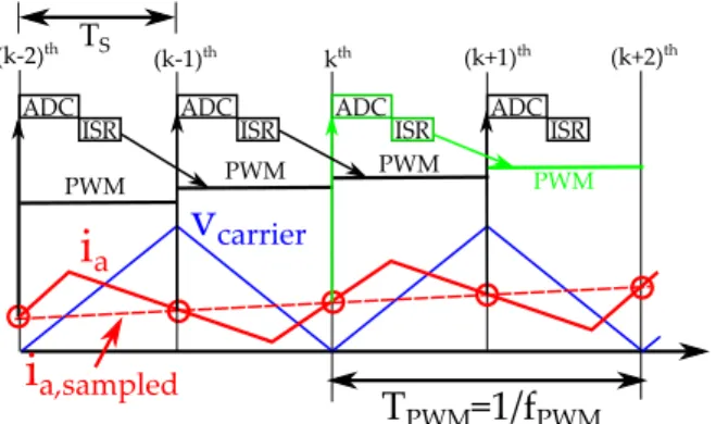
By using carrier based PWM techniques, like SVM as in the current paper, the stator phase currents are synchronously sampled twice at the negative and positive peaks of the carrier signal (see Fig.3) [11]. In this way it can be ensured that, the current is measured in the middle of the zero vector times. In ideal case it provides ripple-free feedback signals for the controllers.

The drawback of the solution is that, the sampling fre- quency is limited and the delay caused by the PWM periph- eral (see later) introduces a phase lag limiting the achievable control bandwidth and deteriorating the performance of the control loop. In general-purpose ac drive applications this effect can be neglected, but it can be crucial, when both the sampling over fundamental frequency ratioF and the carrier over fundamental frequencym_f is low.

It should be noted, in practical drives, the lockout time, the delays of the anti-aliasing filters or the motor cable length can cause additional noise in the current signals even if they are synchronously sampled. Paper [12] introduces a method to avoid these unwanted effects.

In a processor (µC or DSP) based system after the sam- pling and the conversion of the phase currents an interrupt service routine (abbreviated as ISR) is called (Fig.3). In this routine the discrete version of the estimator and the controller algorithms can be found. The controller, based on the measured and the estimated signals, generates the output reference voltagev_s for the induction machine. The PWM algorithm, Space Vector Modulation in our case, calculates the reference signals for each phase. They are latched into the Compare Registers (CR) of the PWM peripheral of the processor to generate the switching signals.

As it was shown previously, estimator algorithms, except for the flux observer based on the stator current, use the value of the stator voltage vectorv_s(in stationary reference frame). In practical applications, the phase voltages are not measured for simplicity and the value of the calculated reference voltage vector is used by estimators.

The sampling of the current signals, the calculation of the estimator algorithm, the control and the PWM algorithm

take less time thanTs. In spite of this, the microcontroller vendor suggests to update the registers of the digital PWM peripheral only in the next half carrier period (see Fig.3).

It means that the voltage reference signals calculated before the negative peak are latched into the CR registers only at the negative peak and vice versa. It results in a constant T_s time delay in the control algorithm between the current sampling and the update of the duty ratios.

ADCISR

i

i

v

PWM PWM PWM

PWM k^th

(k-1)^th

(k-2)^th (k+1)^th (k+2)^th

T

=1/f

T_S

ADCISR

ADCISR ADC

ISR

Fig. 3. Sequence of sampling, calculation and PWM update in a processor based drive system

B. Effect of discretization

At low F ratio the effect of model discretization magni- fies, and some additional errors in the estimation can occur.

According to our findings, one possible source of error can arise from the mismatch between the sampled current and sampled voltage values. Let us assume the estimator reads the current signal at the negativ peak of the carrier signal in thek^thperiod (see Fig.3). Due to the delay in the PWM module, the value of the sampled current was caused by the applied voltage vector which was calculated during the (k−2)^h period. If the estimator algorithm uses the value of the stator voltage vector calculated in the previous(k−1)^th period, a mismatch occurs which can cause error or even instability in the estimator algorithm when the frequency ratio is a low number. This can be avoided by using the voltage vector which belongs to the actual current vector or by predicting the current vector in the next sampling instant.

Another problem, which is crucial at low F ratio, is the phase error between the real and estimated flux or BEMF vectors caused by the discretization and the delay. It can be avoided by adding a compensating angle during the rotation of the vectors. The compensating angle can be assumed to be ωTsorω1Ts, however, depending on the loading conditions this value can change. Paper [3] introduces a controller, which calculates the value of the compensating angle using an integral type controller for MRAS observer.

V. SIMULATION RESULTS

A detailed simulation analysis was carried out using Mat- lab/Simulink environment. The parameters of the machine with rated speed 18 000 rpm can be found in the appendix.

During the simulation the delays occuring in a microcon- troller or DSP based system are also taken into consideration.

A. Flux observers

In this section, the parameter sensitivity analysis of the flux observer based on the stator current and the Gopinath estimator is performed. The parameters under the scope

are the rotor resistanceRr and the mutual inductance Lm. The sampling fs and the switching fc frequency are also changed to demonstrate the effect of the m_f =f_c/f₁ and F =f_s/f₁= 2m_f ratios.

The simulation analysis was performed in open-loop and closed loop as well.

1) Open-loop operation: During this test the machine is supplied by its rated voltage at its rated fundamental frequency (f1= 300Hz) and it is loaded by the rated torque.

To demonstrate and compare the performance of the flux observers the relative error in the estimation of the rotor flux amplitude and the error in the rotor flux angle estimation were calculated in steady state. The first one is calculated as ∆Ψr= ^|Ψr,real_Ψ ^−Ψr,est|

r,real , while the error in the rotor flux angle estimation is obtained as %err =|%Ψ_r,real−%Ψ_r,est|.

Figure 4 summarizes the simulation results for parameter sensitivity in table form. As it can be seen the Gopinath estimator has a much better performance than the flux observer based on the stator current. It is less sensitive on the change in the parameters and estimates both the amplitude and the angle of the rotor flux with good accuracy even at low frequency ratios.

As it can be seen both estimator is more sensitive on the value ofR_r. Based on 4, it is worth to point out that, the magnitude of the error is not the same for positive and negative changes inLm andRr parameters.

(a) Sensitivity of flux observer based on stator current toRrparameter

(b) Sensitivity of flux observer based on stator current toLmparameter

(c) Sensitivity of Gopinath flux estimator toRrparameter

(d) Sensitivity of Gopinath estimator toLmparameter Fig. 4. Simulation results, sensitivity of flux observers at rated speed and at rated loading torque (f1= 300Hz,Mn= 1.6Nm)

Color code: Green (Good): ∆Φr < 5%, %err < 0.08rad, Yellow (Moderate):5%≤∆Φr <10%,0.08rad≤%err<0.15rad, Red (Bad):

10%≤∆Φr,0.15rad≤%err

2) Closed-loop operation: The performance of the flux observers was evaluated in closed loop as well. In this case the machine was controlled by Field Oriented Control method and the flux estimators provided the amplitude and the angle of the rotor flux.

Figure 5 presents the simulated time function of the mechanical speed and the electric torque in closed loop both when the flux observer based on stator current and when the Gopinath estimator was used. The reference speed was selected to be ω∗ = 1750 rad/sec (f₁ ≈ 275 Hz).

The machine loading torque was changed suddenly in both direction. The sensitivity of the flux observer to parameter variation is also tested. Both the value ofLmandRr, which is used in the estimator are changed in both directions.

Figure 5(a) presents the time function ofω andM when the switching frequency was selected to be fs = 3.6 KHz (m_f ≈ 13, F ≈ 26). The value of the rotor resistance used in the estimation was suddenly change by 10%in both direction (see lower diagramm on Fig.5(a)). As it can be seen the vector control works properly for both flux observers.

As it was demonstrated in the previous subsection, the flux observer based on the stator current is more sensitive on the value of Rr. If the rotor resistance used in the estimator is changed by 20% in the negative direction (see Fig.5(b)) the flux observer based on the stator current cannot provide correct results and the closed loop control becomes unstable.

By using Gopinath estimator the system remains stable.

As it was shown previously, the estimators are less sen- sitive on change in the parameterLm. Figure 5(c) presents the simulated Ω and M when the switching frequency is only3 kHz (m_f ≈11, F ≈22) and the value ofL_m used in the estimator is changed by 20% in both direction. The controller works properly in both cases.

B. Speed Estimators

1) Open-loop operation: During this test the machine is supplied by its rated voltage at its rated fundamental frequency (f1= 300Hz).

It should be noted, the PLL-type estimator requires the magnitude of the actual rotor flux (the actual angle of the rotor flux is calculated by the algorithm). During the simulation study, it is provided by the Gopinath estimator.

Figure 6 presents the time function of the real and the es- timated mechanical angular speed, when the loading torque as well as the value of Rr andLm used in the estimation are changed suddenly when the switching frequency is only fc = 3.3 kHz (mf ≈11, F ≈22). The relative error in the speed estimation is calculated as ^ω−ω_ω^est.

As it can be seen both the CB-MRAS and PLL-type speed estimator works properly and the error in the speed estima- tion is less than 1%even when the machine parameters used in the algorithm deviate from the real ones. Comparing the two methods, it can be seen the PLL has a slightly better performance.

2) Closed-loop operation: The performance of the speed estimators was evaluated in closed loop as well. In this case the machine was controlled by Field Oriented Control method and the estimators provided the mechanical speed, as well as the actual rotor flux angle.

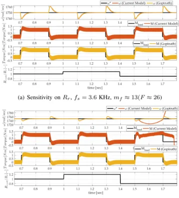
Figure 7 presents the simulated time function of the mechanical speed and the electric torque in closed loop

(a) Sensitivity onRr,fs= 3.6KHz,mf ≈13(F≈26)

(b) Sensitivity onRr,fs= 3.6KHz,m_f≈13(F ≈26)

(c) Sensitivity onLm,fs= 3KHz,mf ≈11(F≈22) Fig. 5. Simulation results, performance of flux observers in closed loop operation

using both speed estimator algorithms. The reference speed was selected again to be ω∗ = 1750 rad/sec (f1 ≈ 275 Hz). The machine loading torque was changed suddenly in both directions. The sensitivity of the speed estimator to parameter variation is also tested. Both the value of L_m andRr used in the estimator are changed suddenly in both direction.

As it can be seen the closed loop control has stable op- eration. The mechanical speed follows the reference speed, the error is around 1%. By comparing the performance of CB-MRAS and PLL-type speed estimators it can be seen the response of the PLL-type estimator became more oscillatory if there is a positive mismatch between the real and the estimated Rr value (see Fig.7(a)). Similarly to the flux observers, the speed estimators are less sensitive on the value of Lm(see Fig.7(b)).

VI. CONCLUSIONS

The paper focuses on high speed drives, where the lowF ratio can be a source of possible error during the discretiza- tion of the estimator algorithms.

(a) Sensitivity onRr,fs= 3.3KHz,m_f ≈11(F≈22)

(b) Sensitivity onLm,fs= 3.3KHz,mf ≈11(F≈22) Fig. 6. Simulation results, performance of speed estimators in open loop operation

(a) Sensitivity onRr,fs= 3.6KHz,mf ≈13(F≈26)

(b) Sensitivity onLm,fs= 3.6KHz,mf ≈13(F≈26) Fig. 7. Simulation results, performance of speed estimators in closed loop operation

The paper introduces the theoretical background of the selected flux and speed estimator techniques. The discrete- time equations of each algorithm is derived by using Tustin approximation. The discrete form of each algorithm can be implemented by the recursive equations presented in this paper.

The performance of the algorithms both in open and closed loop is validated via numerical simulation using a high speed motor drive with a low sampling to fundamental frequency ratio.

Another paper will discuss the laboratory measurements with additional information on the practical implementation.

APPENDIX

The rated data and main parameters of the machine are: power:

PN= 3kW,ULL,RM S= 380V,IN,RM S= 7.7A,f1N= 300Hz, RS = 1.125Ω,RR= 0.85Ω,XLS = 4.71Ωand XLR= 2.63Ω, Xm= 84.82Ω(all reactance are at rated frequency),p= 1

REFERENCES

[1] A. Tenconi, S. Vaschetto, and A. Vigliani, “Electrical machines for high-speed applications: Design considerations and tradeoffs,”IEEE Transactions on Industrial Electronics, vol. 61, no. 6, pp. 3022–3029, June 2014.

[2] K. S. Kim and I. H. Kim, “Design of a discrete flux observer by the power series approximation,”Journal of Power Electronics, vol. 11, no. 3, pp. 304–310, March 2011.

[3] D. Marcetic, I. Krcmar, M. Gecic, and P. Matic, “Discrete rotor flux and speed estimators for high-speed shaft-sensorless im drives,”

Industrial Electronics, IEEE Transactions on, vol. 61, no. 6, pp. 3099–

3108, June 2014.

[4] B. Wang, Y. Zhao, Y. Yu, G. Wang, D. Xu, and Z. Dong, “Speed- sensorless induction machine control in the field-weakening region using discrete speed-adaptive full-order observer,”IEEE Transactions on Power Electronics, vol. 31, no. 8, pp. 5759–5773, Aug 2016.

[5] T. O.-K. Mateusz Korzonek, “Application of different numerical integration methods for discrete mras-cc estimator of induction motor speed comparative study,” inIEEE PEMC 2018 18th International Conference on Power Electronics and Motion Control, 2018, pp. 808–

8013.

[6] N. T. West and R. D. Lorenz, “Digital implementation of stator and rotor flux-linkage observers and a stator-current observer for deadbeat direct torque control of induction machines,”IEEE Transactions on Industry Applications, vol. 45, no. 2, pp. 729–736, March 2009.

[7] T. Orlowska-Kowalska and M. Dybkowski, “Stator-current-based mras estimator for a wide range speed-sensorless induction-motor drive,”

IEEE Transactions on Industrial Electronics, vol. 57, no. 4, pp. 1296–

1308, April 2010.

[8] Y. B. Zbede, S. M. Gadoue, and D. J. Atkinson, “Model predictive mras estimator for sensorless induction motor drives,”IEEE Transac- tions on Industrial Electronics, vol. 63, no. 6, pp. 3511–3521, June 2016.

[9] H. H. Vo, P. Brandstetter, and C. S. T. Dong, “Mras observers for speed estimation of induction motor with direct torque and flux control,” inAETA 2015: Recent Advances in Electrical Engineering and Related Sciences. Springer, 2016, pp. 325–335.

[10] I. Krcmar, P. Matic, and D. Marcetic, “Discrete rotor flux estimator for high performance induction motor drives with low sampling to fundamental frequency ratio,” International Review of Electrical Engineering, vol. 7, pp. 3804–3813, Aug 2012.

[11] J. O. K. C. Klarenbach, H. Schmirgel, “Design of fast and robust current controllers for servo drives based on space vector modulation,”

inPCIM Europe 2011; International Exhibition and Conference for Power Electronics, Intelligent Motion, Renewable Energy and Energy Management, 2011, pp. 182–188.

[12] S. N. Vukosavic, L. S. Peric, and E. Levi, “Ac current controller with error-free feedback acquisition system,”IEEE Transactions on Energy Conversion, vol. 31, no. 1, pp. 381–391, March 2016.