Óbuda University
PhD Thesis
Design of processes supporting the development of medical devices
by
József Klespitz
Supervisor:
Prof. Dr. habil Levent Kovács
Applied Informatics and Applied Mathematics Doctoral School
Budapest, 28
thFebruary 2018
Declaration of Authorship
I, József Klespitz, declare that this thesis titled, ’Design of processes supporting the development of medical devices’ and the work presented in it are my own. I confirm that:
• This work was done while in candidature for a research degree at this University.
• Where I have consulted the published work of others, this is always clearly attributed.
• Where I have quoted from the work of others, the source is always given. With the exception of such quotations, this thesis is entirely my own work.
• I have acknowledged all main sources of help.
_______________________
PhD Candidate
_______________________
Date
Contents
1 Introduction ... 1
1.1Research focus ... 1
2 Control of hemodialysis machines ... 3
2.1 Technical background ... 3
2.2 Model of controlled system ... 5
2.3 Fuzzy controllers ... 8
2.3.1 Design of the controllers ... 8
2.3.2 Iterative Learning Control for fuzzy controllers ... 12
2.3.3 Performance of fuzzy controllers... 16
2.3.4 Evaluation in real environment ... 18
2.4 Adaptive Neuro-Fuzzy Inference Systems ... 19
2.4.1 Training sets... 20
2.4.2 Controller design ... 20
2.4.3 Evaluation of controller performance ... 21
2.4.4 Evaluation on real machine ... 24
2.5 LMI-based feedback regulator ... 26
2.5.1 Controller design ... 27
2.5.2 Evaluation of the controller ... 29
2.5.3 Verification in real environment ... 30
2.6 Conclusions ... 31
3 Application lifecycle management system improvements ... 35
3.1 Basics of application lifecycle management systems ... 35
3.2 Heterogeneous and homogeneous ALM systems ... 37
3.3 Traceability and Consistency ... 40
3.4 Augmented Lifecycle Space ... 43
3.5 Demonstration of Augmented Lifecycle Space approach .... 46
3.5.1 Application practice ... 46
3.5.2 Homogeneous test system ... 47
3.5.3 ALS for homogeneous system ... 50
3.5.4 Analysis and detections ... 51
3.5.5 Industrial feedback on results ... 60
3.5.6 Summary of the homogeneous case ... 61
3.6 Demonstration for heterogeneous ALM system ... 62
3.6.1 Used tools and system setup ... 62
3.6.2 Analysis in collaboration ... 64
3.6.3 Result and feedback for heterogeneous case ... 66
3.6.4 Summary for heterogeneous case ... 69
4 Summary ... 71
5 Bibliography ... 72
5.1 References ... 72
5.2 Own publications pertaining to Thesis ... 80
5.3 Other publications Not Pertaining to Thesis ... 81
Acknowledgements
First of all, I would like to thank my doctoral supervisor, Prof. Levente Kovács – he was the one who gave me the encouragement to continue my studies and he was the one also who smoothed my way during these times. He taught me that everything is possible with full devotion and hard work.
Next, I would like to say thank to Dr. Márta Takács for her helps regarding fuzzy systems.
Without her potent help it would be more cumbersome to execute the experiments.
After, I would say thank to Dr. Miklós Bíró who has taught me the scientific presentation of software technology. He was the one who came up with the idea of Augmented Lifecycle Space which is the base of my second thesis group. I am glad for his patience and accuracy what he has shown towards me during our collaboration.
I am very grateful for B.Braun Medical Ltd. with specific regard to the late Dr. Sándor Dolgos. He not only let me use the results achieved at the company, but he also supported my studies in every aspect. I will keep his attitude towards other people, and his humanity towards the colleagues.
Special thanks behoove the Doctoral Shool lead by Prof. Aurél Galántai and the Research and Innovation Center of Óbuda University lead by Prof. Imre Rudas.
It was a pleasure to work in the Physiological Control Research Center. Thank you guys for every help and keep up the good work! I wish to thank especially the help provided by Johanna Sápi Sájevicsné, Tamás Ferenci, and György Eigner. You made everything easier.
I would like to also thank to all of those who are not personally listed here – many of my colleagues and friends from whom I learned a lot.
Finally, I want to say thanks to my family, this work would have been impossible without their help and support. Without the stimulation of my Mom and Dad, it would take much longer time to do this work. They were the ones who taught me the importance of studying.
I would like to say special thanks to my wife Kriszti. She was always there when needed and she was the one who kept my enthusiasm. She is the light in my life and everything would be much more boring and quiet without her.
The thesis reported in this paper has been partially supported by the Austrian Ministry for Transport, Innovation and Technology, the Federal Ministry of Science, Research and Economy, and the Province of Upper Austria in the frame of the COMET center SCCH.
List of Figures
1. Figure Analyzed subsystem ... 6
2. Figure Model of the controlled system ... 7
3. Figure Surface map of the fuzzy controller ... 12
4. Figure Original model of iterative learning control ... 14
5. Figure Internal structure of adaptive fuzzy controller ... 15
6. Figure Membership functions covering the input of controller ... 15
7. Figure Result on target machine with adaptive fuzzy controller ... 18
8. Figure Internal structure of ANFIS ... 19
9. Figure Modified ANFIS structure with ILC ... 21
10. Figure Bode-diagram of modified ANFIS structure ... 23
11. Figure Results with modified ANFIS controller on target machine ... 24
12. Figure Weighting functions ... 29
13. Figure Result of PI controller on the target machine ... 31
14. Figure Content of an Application Lifecycle Management System ... 37
15. Figure Traceability and consistency relationships in Automotive SPICE v3.0 ... 43
16. Figure Traceability and consistency relationships from Automotive SPICE featured in this research ... 47
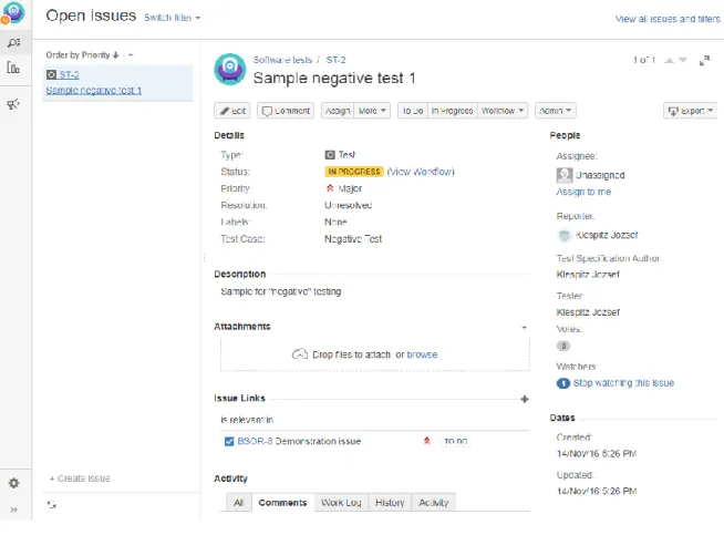
17. Figure Example requirement „issue” ... 48
18. Figure Example „issue” with issue links ... 52
19. Figure Defected issue with missing links ... 53
20. Figure Workflow generated automatically to fix missing linking ... 54
21. Figure Example test requirement for out-of-bound test case ... 55
22. Figure Parent requirement of previous test showing test coverage ... 56
23. Figure Outdated issue ... 57
24. Figure Workflow generated for reviewing outdated item... 58
25. Figure Overview of featured problems ... 59
26. Figure Generic workflow scheme ... 60
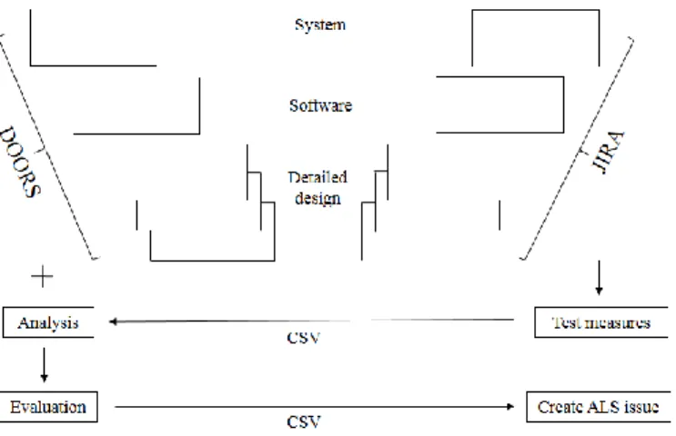
27. Figure Information flow in heterogeneous system analysis ... 66
28. Figure Generated workflow in heterogeneous system with reference to the place of finding ... 67
List of Tables
Table I. Settling Time ... 16
Table II. Overshoot ... 17
Table III. Accuracy ... 17
Table IV. Settling time results ... 22
Table V. Overshoot results ... 22
Table VI. Accuracy measurement results ... 23
Table VII. Measurement on the real system ... 25
Abstract
Hemodialysis machines are responsible for removing metabolic waste products from the human blood when the body cannot excrete them on its own. With their help it is possible not only to improve the life quality of patients with kidney malfunction, but in certain cases this is the only way to keep someone alive.
The software component in these machines has significantly improved with the accessibility of powerful computing devices. Not only the expectations of experts has changed (more accurate device, improved patient safety, cost efficient operation), but also the international regulations have been modified. Altogether, these facts raise a challenge for development teams. In this thesis I am analyzing two aspects of the aforementioned problems.
During treatment, the blood of the patient is extracted and filtered extracorporeally. The purification is done by using special dialysis fluids where at the end, excess fluid is removed.
This means that the fluid transfers have to be supervised to keep the patient fluid balance.
Soft computing methods were developed and compared with conventional control methods in the first thesis group. This approach is novel for the industry and analyzes have proved it to be effective. The developed controllers are comparable with the existing solution with the advantage of possible incorporation of additional expert knowledge. The controllers were developed to be not only suitable for testing and analyzes, but they can be easily integrated into existing machines.
The quality of a newly developed machine is highly depending on the applied development process. Different supporting tools are used to decrease documentation related burden, eliminate redundancies and to reduce human workload. The tools in the development toolchain are called application lifecycle management system and they can be homogeneous or heterogeneous depending on the number and connectivity of software providers. The second thesis group discusses how enhanced traceability and consistency can be achieved when using these systems. The idea of augmented lifecycle space was created as a software independent solution to find missing artifacts in software development. Furthermore, it makes possible for stakeholders to select and prioritize the deficiencies.
Absztrakt
A szükségtelen anyagcsere termékeket hemodialízis készülék segítségével lehet eltávolítani az emberi vérből. Segítségükkel a veseelégtelenségben szenvedőknek nem csak az életminőségét lehet így javítani, hanem bizonyos esetekben ez az egyetlen mód az életben tartásukra.
Ezen gépek szoftver komponense jelentősen fejlődött a nagy teljesítményű eszközök terjedésének köszönhetően. Nem csak a szakértő felhasználók elvárásai (úgymint pontosabb eszköz, magasabb betegbiztonság, költséghatékony működtetés) emelkedtek, hanem a nemzetközi szabályozások is változtak. Mindezek együtt kihívás elé állítják a fejlesztő csapatokat. Jelen disszertációban a korábban említett problémák két aspektusát vizsgálom.
Kezelés közben a beteg vérét kinyerik és a testen kívül megszűrik. A megtisztítást speciális dialízis folyadék segítségével végzik, ahol is a felesleges folyadékmennyiséget eltávolítják.
Ezért a beteg folyadékegyensúlyának megtartása érdekében a folyadék áramlásokat felügyelni kell. Az első téziscsoport a lágy számítási módszerek fejlesztését és hagyományos módszerekkel való összehasonlítását tartalmazza. Az így fejlesztett szabályozók összehasonlíthatóak a meglévő megoldásokkal, miközben megvan az az előnyük, hogy szakértői tudással bővíthetők. A szabályozókat nem csak tesztelési és analitikai célokra lehet használni, hanem könnyen integrálhatóak meglévő gépekbe.
Egy újonnan kifejlesztett gép minősége nagyban függ az alkalmazott fejlesztési folyamatoktól. Különböző támogató eszközök alkalmazhatóak a dokumentációs terhek csökkentésére, illetve az emberi terhelés csökkentésére. A fejlesztési eszközláncban található eszközöket együtt applikációs életciklus menedzsment rendszernek hívják, ami lehet homogén vagy heterogén a benne található szoftverek számától és összekötöttségétől függően. A második téziscsoport azt tárgyalja hogyan lehet a nyomon követhetőséget és konzisztenciát növelni ezen rendszerekben. A kiterjesztett életciklus tér, mint egy szoftver független megoldás, a hiányzó fejlesztési artifaktok megtalálására érdekében lett kifejlesztve. Mi több, segítségével a döntéshozók a hiányosságokat válogathatják és fontossági sorrend szerint rendezhetik.
1
1. Introduction 1.1. Research focus
This doctoral thesis is related to hemodialysis machines, their operation and their development. Hemodialysis machines are used to replace or support the kidney functionality during malfunction which process is known as blood purification. Renal replacement therapies are required in case of kidney malfunction which can be grouped as acute and chronic kidney failure. It is also used to improve quality of life until the kidney of the patient could be transplanted. The need for such machines is well demonstrated by showing that chronic kidney disease is the 9th leading death cause in the United States [1].
Chronic kidney disease is built up over a longer period of time while the glomerular filtration ratio (blood purification capability of kidney) is gradually decreasing. After a certain threshold, the kidney cannot remove enough metabolic waste products and it begins to accumulate in the body. The accumulation of these waste materials results unpleasant symptoms (fatigue, drowsiness, itching, joint pain) in the beginning, but it could achieve life threatening conditions as well [2].
This makes it inevitable to remove the waste products by blood purification. In case of chronic kidney disease these treatments have to be repeated multiple times a week where each treatment lasts for 4-6 hours. The treatments get more frequent with the weakening performance of kidney. In the end kidney transplantation is inevitable and also this is the only permanent cure for chronic kidney disease [3]. The chronic kidney disease is spreading, estimated to affect more than 10% of adults in the United States, elder people over 70 years are especially threatened [4].
On the other hand, acute kidney injury is the rapid loss of kidney functionality. It is caused by a trauma with a variety of backgrounds [5]. According to Susan et al. [6] every one in five adults and one in three children experiences acute kidney injury in hospital care.
Critically ill patients are especially threatened and their mortality is significantly affected by the presence or absence of renal replacement therapy [5].
Acute kidney injury typically lasts for hours or days. If the injury does not recover (at least partially) within 3 weeks then it is considered chronic kidney disease. The chance of recovery depends on the cause and the severity, for further information see Bellomo et al.
[5]. It is crucial to use renal replacement therapies upon indication [7] to improve outcome, to decrease excess hospital costs and to enhance the chance of kidney function recovery [8].
In case of acute kidney injury a so called continuous renal replacement therapy is used. Here, the blood purification is continuous and it can lasts over 72 hours as the patient’s condition requires.
By looking at statistics, the hospitalization need and the morbidity is slightly decreasing in the United States, while the overall occurrence of chronic kidney disease is stagnating thanks
2
to the healthcare system and prevention [9]. Detailed demographics can be found at [10].
Although most metrics are available only regarding the United States, still further estimation can be done. The increasing occurrence of kidney failure is expected in both developed and developing countries as diabetes and high blood pressure, the two important pandemics, are the leading causes of kidney failure [1] [11]. Due to these facts together with the limited possibility of kidney transplantation (which is the one and only final cure in end stage renal disease) it is clear that these patients has to be taken care of. Altogether, this raise the need for modern and economic hemodialysis machines to prolong the life and to improve the living conditions of patients.
As it was shown above, the blood purification treatment is different in case of the two diseases. Although, the facility need is different, yet the phenomena behind each therapy is similar [12]. The blood of the patient is removed via a cannula and it is flowing through a tubing system extracorporeally. Hereby, the blood is running through a capillary system (filter), where capillaries are made from semipermeable membrane. The waste materials are removed via this membrane with various methods [13].
When there is a counter flow of dialysis fluid on the other side of semi-permeable membrane and waste material is removed via diffusion then the therapy is called hemodialysis. When there is no dialysis fluid on the other side of the semi-permeable membrane and the pressure difference forces part of the blood through the membrane creating the so called ultrafiltrate then it is called hemofiltration. When there is also a counter flow of dialysis fluid and the pressure difference also secretes ultrafiltrate then the therapy is called hemodiafiltration.
Each therapy type has its own indication. When ultrafiltration is created then it is necessary to replace the removed fluid volume. This is solved by administering dialysis fluid to the blood of the patient. In each cases, the purified blood is flowing through an air trap to remove air bubbles from the blood before introduced back into the body.
Acute hemodialysis machines are usually mobile (to let them move between intensive care units), the necessary fluids are stored in different bags and also the waste products are collected in separate bags. On the other hand, the chronic machines (where the mobility is not an issue) are connected to a small dedicated water plant and the machine creates itself the dialysis fluids and transfer waste materials to the sewers.
Although the principles of hemodialysis is simple and it has not changed significantly over its century old history, still it is not self-evident to launch a new device on the market. First of all it is a medical device thus it is capable to harm (and even kill) someone. Therefore, it is a safety-critical application where the related standards and directives has to be fulfilled and the manufacturer has to guarantee the safe operation. Tremendous amount of documentation and proper processes are needed to develop successfully a machine while continuously considering and avoiding possible risks and hazards. The documentation burden and process control is supported by various software tools. To ease this job many tools can be found on the market even with some solutions dedicated to the medical device
3
domain. The communication and information share between these applications is a crucial point, where further improvements are still needed.
The dissertation is organized around two problems. First, it will be discussed how the patient fluid balance can be kept by controlling the fluid pumps in the system. Hereby, soft- computing methods are analyzed as a novel application field together with other control methods mostly unknown for the industry.
However, it is not satisfactory to only insert a suitable controller in the machine software, but it has to meet every requirement while complying the specified development processes.
The second part will discuss this topic: Namely, how a software development can be supported by different tools and how the transparency and quality of development could be improved with little to no human interaction. Thus, the application of a novel method is demonstrated which is capable to find deficiencies and it also provides a workflow automatically in order to get rid of these problems.
2. Control of hemodialysis machines 2.1. Technical background
In hemodialysis machines peristaltic pumps are responsible for fluid transportation including blood of the patient [12]. They are transporting liquids by repeatedly compressing an elastic tube(segment) without getting in contact of the transferred fluid. Peristaltic pumps can be operated with disposable tubing which is practical as the treated blood gets in contact only with the sanitized kit. This way infection and contamination can be avoided. Furthermore, the tubing of treatment kit can be created from biocompatible materials. This way the chance of (blood) coagulation can be reduced together with the chance of filter clogging without even using anticoagulation materials. Finally, peristaltic pumps are gentle to the transported fluid. This is especially important in case of blood, as the breakdown of corpuscles (formed elements) should be avoided. From medical point of view the only drawback of peristaltic pumps is their inaccuracy.
Hemodialysis machines typically operate with two roller peristaltic pumps (at least for the main pumps). The operation of such a pump can be characterized as the following: At the beginning of the sequence the first roller closes the tubing inlet. Afterwards, the roller moves forward and pushes the pump segment to the manifold. This way it pushes the fluid inside the tube forward and generates a pressure wave. Before reaching the outlet the other roller closes the tube inlet, this way it prevents the black-flow. After the first roller leaves the outlet, the other roller's task will be to generate the next pressure wave. This sequences repeats over time and this creates a continuous flow in the tubing. More details can be read about peristaltic pumps at [KJ2].
4
During treatment the blood is partially re-exchanged with dialysate fluid, but excess body fluid can also be removed. However, the balance between total amount of given and removed fluids has to be the same as specified by the doctor (typically a negative amount of fluid to support the lacking secretion of body). This prescription is defined as net fluid removal and it is defined as flow rate [ml/h] which might change throughout the treatment. The actual removal can be bigger or equal to zero in spite of the above. If the kidney of patient is capable to remove satisfactory amount of water and only the clearance has to be supported then this amount is zero. If the kidney cannot remove enough water or other indication exists then the actual value is defined by doctors according to current needs.
This is one of the most crucial aspects of these machines as removing excess fluid is necessary to improve health of patient. On the other hand, removing too much fluid can lead to dehydration which might increase to a life threatening level. (Not to mention that it is guaranteed that it further burdens the already bad general condition of the patient.) Furthermore, in certain machines peristaltic pumps are also used for transporting drugs.
Heparin might be administered for prevention of anticoagulation or calcium replacement might be necessary when it is removed with citrate complex, again for anticoagulation purposes. The precise transfer is even more crucial in such cases as overdosing, hypocalcaemia or hypercalcaemia may occur. Altogether, this raise the need for regulation and supervision of fluid transport.
In case of acute hemodialysis machines, the different liquids (such as the dialysate, or effluent fluids) are collected and treated in different bags. This is necessary to keep the machine mobile, to let it move between different premises (operating rooms, intensive care units, etc.). This way no external water supply is necessary. The fluids (dialysate and substitution fluids) are removed from these bags, while the effluent fluid is collected similarly. This way, the fluid transports can be measured with weighting scales. With the comparison of measured and desired fluid volumes it is possible to calculate delivery errors.
(The idea can be utilized for chronic hemodialysis machines as well, but it is more difficult to measure the transferred volume in the absence of fluid bags and separate weighting scales.)
The inaccuracy of peristaltic pumps is the main reason of feed-back control [14]. The elasticity of tube segment may result approximately ± 10% in total transferred volume due to deviation of production [15]. Furthermore, the transferred volume is depending on pressure ratio which might further worsen the fluid balance. The accumulation over the long therapy time (up to and over 72 hours) could further increase these effects. The fatigue of tubing material has to be also mentioned. The continuous repeated squeezing of the material will make it stiffer over time. Thus, it will be unable to reshape completely to its original form which also means that the inner volume (thus the transfer volume) gets decreased.
Finally, pressure ratios may alter the volume of elastic tube segment. By increasing the pressure ratio it is capable to force more fluid into the tube segment, “blowing it up like a balloon”. This means increased transfer volume. On the other hand, decreased pressure ratio
5
hinders the filling of the tube segment in a way that during relaxation it is not filled to its full capacity. Naturally, this decreases the transfer volume. From these two phenomenon the negative pressure ratio is the more relevant, as such pressure levels can be practically reached. The other (positive) case is less common, but it has to be still kept in mind. Either way, both of these phenomenon develops out of normal operating range. Therefore, the controller has to be prepared for these cases, but the expectations are different compared to normal operation mode (i.e. less control reserve).
Many complex approaches can be found in the literature about controlling hemodialysis machines. Most of these (e.g. [16, 17, 18, 19]) are estimating techniques where a set of physiological parameters (e.g. arterial blood pressure, heart rate, blood density, etc.) are selected and used to override therapy parameters. This seems to be promising, but at the moment manufacturers do not take the risk of letting the intervention decided by the machine. Machine calculations are only used for decision support and the final decision is made by the expert. This way the aforementioned systems remain promising but they are not available on the market. (Still, it is an interesting thought to have self-setting machines which are tuning treatment parameters to the actual need of the patient. This could be as exciting step as a completely autonomous car in traffic.)
It has to be mentioned that patient fluid balance control is not the only place where feedback control is necessary. The different pressure ratios shall be kept between certain boundaries mostly to prolong the life of the filter and ease the operation of peristaltic pumps.
Furthermore, the temperature of the blood has to be maintained as it is cooling extracorporeally. This can be also used to improve patient comfort as the temperature of re- introduced blood affects the temperature sensation of patient.
This part of thesis targets to demonstrate the use of non-conventional control methods for regulating patient fluid balance via peristaltic pumps. First soft computing methods and their performance will be presented. Afterwards, the design of a classical PI controller will be shown by using tensor product transformation. Each of the designed controllers should be suitable for real-life application with possibility of integration into an existing machine.
2.2. Model of controlled system
One pump and its related tubing with fluid bag was separated as a subsystem as Figure 1 presents. The pumps could be analyzed altogether as a single multi-input multi-output (MIMO) system. However, this idea was neglected, as the testing (and generally the verification and validation procedure) would be more demanding. Furthermore, the correlations between the pumps can be neglected as a good approximation without risking the compliance of performance requirements. Thus, the more simple single-input single- output (SISO) approach was supported. In this case the controller of subsystems eliminates errors of the corresponding pump and in summary this will result the accurate transportation from systemic point of view.
6
1. Figure Analyzed subsystem
The separated subsystem consists a peristaltic pump responsible for the fluid transport, a bag responsible for granting or collecting the fluid and a weighting scale responsible for measuring transferred fluid weight. This subsystem was identified with specific regards to insecurity in fluid transport volume, quantitation error of weighting scale and the insecurity of rotation of pump head [KJ1]. Although, multiple advanced identification model were used (namely ARX, ARMAX and Box-Jenkins), still the single state-space model was the most accurate model which resulted the following transfer function:
H(s) = Kpump/s (1)
By identifying the Kpump amplification, the root mean square error was measured 0.13% as percentage of full scale (or 1.3 grams). This could be caused by the simplicity of subsystem and the time invariant property of the selected subsystem.
The final model of the analyzed system can be seen on Figure 2. Here, two main branches can be distinguished. Each branches contain the identified transfer function. The first branch is responsible for the ideal transfer volume, also this is the reference signal. Therefore, the transfer function is unchanged in the first branch. The second branch is responsible for the real transfer volume which includes the possible errors and distortions. It starts with a gain responsible for slope errors. Here, the tube related errors can be introduced (fatigue, pressure dependency, tube inaccuracies and rotation dependency). This is followed by the transfer function. After that, constant can be added to the system, responsible for the different weight measure errors. Simulation of single weight error and residual error can be executed with its help.
7
2. Figure Model of the controlled system
The output of the model is equal with this second branch. The difference of the estimated transfer volume (first branch) and real transfer volume (second branch) is the error signal.
This error signal is provided for the controller which creates the feedback signal. This signal is fed back via a glue logic to the second branch to compensate its inaccuracy. The glue logic (and the positive feedback) is similar to a practical implementation to make the integration of the analyzed controllers possible.
This model has the benefit of the generic controller which can be replaced with any selected controller. Initially, a PID controller was inserted and for the other measurement the results of this controller meant the benchmark. The integral term is necessary as the residual error means fluid imbalance in the body of the patient which cannot be tolerated. The derivative term is only necessary to reduce the settling time to reach tight control.
The following properties of the controllers were analyzed:
settling time
overshoot
accuracy
robustness
Each of these have a physiological meaning and relevance. Let them see in order: settling time shall be minimized as the error of a pump means fluid imbalance in the body. It is important to minimize the time with fluid imbalance, but it can be tolerated most of the time as the human body is robust from this perspective. However, it is vital to minimize this time when the effluent pump is transferring drugs as the effect of deviation can be more destructive in such cases. The overshoot means unnecessary burden for the patient, thus it
8
needs to be avoided at all if possible. The accuracy is a long term goal which reduce the time and amount of fluid imbalance. Finally, robustness is necessary to handle uncertainty in the system such as the volume of elastic tube segment, the fatigue of this tube and delivery fluctuation caused by pressure.
2.3. Fuzzy controllers
In the following chapters the designed controllers are presented together with the achieved results. The reference is always the PID controller as one of the motivation of this research is to prove for industrial developers that the performance of soft computing methods can be equal or even better in safety-critical environment. The aforementioned reference PID controller [KJ1] was designed for a 61° phase margin [20]. Later on this is used always as a base for comparison. Moreover, some selected controllers were tested in a real hemodialysis machine too. Thus, the results of comparison got verified as well.
2.3.1. Design of the controllers
First of all, a simple fuzzy controller was created. Mamdani-type fuzzy controller was chosen for the implementation as they are closer to the human thinking and the task was basically capturing the system related expert knowledge [21]. The computational efficiency was not a target in the initial phase as the aim of the research was to show the usability of fuzzy logic in the given environment [22]. Moreover, the used tool (Matlab) has a dedicated command for transforming Mamdani-type systems to Sugeno-type system. This way, if the controller proves to be effective then it is still possible to utilize the efficiency of Sugeno-type systems later during the implementation.
Originally, a simple fuzzy controller was designed with a single input as the base of research.
At that time, there were no requirements about the strictness of control and intervention.
Thus a fine resolution was applied on the single input signal of the system which was the transfer volume error. The error signal was covered by 19 membership functions weighted from 1% to 50% with the following pattern: 1%-2%-5%-10%-20%-etc. Intermediate regions were covered by triangular-shaped membership functions characterized by:
𝑓(𝑥) = {
0, 𝑖𝑓 𝑥 ≤ 𝑎
𝑥−𝑎
𝑏−𝑎, 𝑖𝑓 𝑎 ≤ 𝑥 ≤ 𝑏
𝑐−𝑥
𝑐−𝑏, 𝑖𝑓 𝑏 ≤ 𝑥 ≤ 𝑐 0, 𝑖𝑓 𝑐 ≤ 𝑥
(1)
where a and c characterize the region where the f function is non-zero and it is assumed that a ≠ b and b ≠ c. The values of a and c are selected for each membership function in a manner that their overlapping sequence intersects only the adjacent membership functions.
Furthermore, the defined regions by a and c are increasing continuously proportionally with the error signal. To guarantee the symmetry let = 𝑎+ 𝑐2 . The centers of 19 membership functions are belonging to error 0, ±1, ±2, ±5, ±10, ±20, ±50, ±100, ±200 grams of delivery
9
error. None of the membership functions cover transfer volume errors over ±500 grams.
These values were based on initial consideration and worst case scenario calculations. Later, these assumptions got rejected in spite of the first results.
The two end regions were covered individually with unique membership functions. Transfer volume errors below -500 grams were covered by a z-shaped membership function characterized by:
𝑓(𝑥) = {
1, 𝑖𝑓 𝑥 ≤ 𝑎
1 − 2 (𝑥−𝑎𝑏−𝑎)2, 𝑖𝑓 𝑎 ≤ 𝑥 ≤ 𝑎+𝑏2 2 (𝑥−𝑏𝑏−𝑎)2, 𝑖𝑓 𝑎+𝑏2 ≤ 𝑥 ≤ 𝑏
0. 𝑖𝑓 𝑥 ≥ 𝑏
(2)
where a is the limit of maximal (considered) transfer error based on acquired knowledge and a-priori information. b is reasonably close value to guarantee the steepness of the transition.
Transfer volume errors above 500 grams were covered by an inverse z-shaped function characterized by:
𝑓(𝑥) = {
0, 𝑖𝑓 𝑥 ≤ 𝑎
2 (𝑥−𝑎𝑏−𝑎)2, 𝑖𝑓 𝑎 ≤ 𝑥 ≤ 𝑎+𝑏2 1 − 2 (𝑥−𝑏𝑏−𝑎)2, 𝑖𝑓 𝑎+𝑏2 ≤ 𝑥 ≤ 𝑏
1. 𝑖𝑓 𝑥 ≥ 𝑏
(3)
where b is the limit of maximal (considered) transfer error based on acquired knowledge and a-priori information. a is reasonably close value to guarantee the steepness of the transition.
The error signal is normalized by the used tool (Matlab), and T-norm is used to calculate the result of membership functions:
𝑇(𝜇𝐴(𝑥), 𝜇𝐵(𝑥)) = 𝜇𝐴(𝑥) ∗ 𝜇𝐵(𝑥) (4)
where μA and μB are the affected membership functions and * means the minimum of μA(x) and μB(x).
The initial result were unsatisfactory with this setup. First of all, this controller was unable to remove the residual error from the system. On the long run this cannot be tolerated, its elimination is mandatory. Furthermore, it is a vital aspect for the controller to find the exact operating point for the elastic tube segment. This kind of adaptivity is necessary, to set the reserve accordingly. This means that the control range (coming from directives) is defined in the range of real transfer volume. The better we can set this volume, the more reserve the system have. Thus, the error can be removed faster.
These needs have two additional reasons as well. First of all, the tube will age throughout the therapy and this decreased elasticity will result in less transfer volume, the operating
10
point will be shifted. The adaptivity is important to follow this, and keep the control range as wide as possible. The other phenomena explains the need for the wide control range: both the increment and decrement of the systemic pressure can affect the transfer volume significantly. Moreover, this pressure might change suddenly (compared to the velocity of system) thus introducing error into the transfer. The wider range we have the better we can compensate this and other disturbing effects in order of the improved patient service.
To solve these problems two other fuzzy controllers were created one with integrating property and another one which is capable to adapt.
At first the problem of residual error was targeted. Just like in case of the PID controller an integral term is necessary to solve this. The usage of the integral of error signal was unsuccessful due to instabilities. This way the solutions were combined and the number of inputs of fuzzy controller was increased. At first, the introduction of a derivative term seems to be useful as well in order to have an estimator. Unfortunately, this is impractical as the error is based in weight calculation where the resolution of weight measurement is 1 gram.
This is in the range of real errors and it is impossible distinguish them. Therefore, the introduction of a derivative term only decreases the performance due to the wrong predictions [23].
It was clear from the results of original fuzzy controller that the number of membership functions can be highly reduced and the considered range of the error signal can be decreased. These can be done due to the facts, that most of the reactions for various membership functions/certain regions could not been distinguished and with a proper controller during normal operation not even the ±100 range was exceeded. (Otherwise, in certain scenarios error over this threshold can be reached, but these are special situation where reaction for maximal error is suitable to handle these cases as well.)
In spite of the above mentioned facts the error signal was covered by seven membership functions during fuzzyfication. The intermediate five functions were triangle shaped membership functions as described in Eq. (1). These were distributed equidistantly between the selected extremities (±50 gram), in a manner that membership function might intersect only their adjacent membership functions. The only exception is the central function responsible for minimal to no error. This one was a tighter function centered on 0. This function was referred later as “MinErr”, while the other ones were generated from the big/small and positive/negative word pairs. The terminal membership functions were changed to trapezoidal membership functions characterized as:
𝑓(𝑥) = {
0, 𝑖𝑓(𝑥 < 0) 𝑜𝑟 (𝑥 > 𝑑)
𝑥−𝑎
𝑏−𝑎, 𝑖𝑓 𝑎 ≤ 𝑥 ≤ 𝑏 1, 𝑖𝑓 𝑏 ≤ 𝑥 ≤ 𝑐
𝑑−𝑥
𝑑−𝑐, 𝑖𝑓 𝑐 ≤ 𝑥 ≤ 𝑑
(5)
11
where c was selected as -50 grams for the negative extreme as the maximum error to consider (based on experiences with previous fuzzy controller), and b was selected as -200 grams as them maximum possible error to be tolerated (above this safety measures are required according to directives) a and d are selected to be somewhat lower than b and c respectively in a way to provide the necessary slope. Similarly, on the positive extreme the b was selected as 50 grams and c was selected as 200 grams just like in case of the negative extreme. a and d was selected in the same manner as well.
The other input, the integral of error signal was covered with five membership functions.
Due to the high quantitation error it was known that the range should be increased compared to the error signal and the small values did not need finer coverage. The intermediate membership functions are triangle shaped as described in Eq. (1) and they covered the full range equidistantly. Names used during fuzzyfication are referring to these as “Minimal”,
“Positive” and “Negative”. The other two membership functions are trapezoid membership functions as described in Eq. (5). The trapezoid membership functions outreach the thresholds by ±200 g (determined empirically) and the integral of error signal is also saturated at ±200 g. Saturation was necessary as the system would be otherwise capable to accumulate significant amount of error which is not desired, as it might cause high overshoot and significantly longer transient time (this is the so called windup phenomenon). Anti- windup systems are commonly used in PID controllers and it is highly advised to use one in this very situation. This will prevent the unnecessary increase of the integral of error if the control signal is in saturation. In order do this the output and the saturated value of the output are compared. A switch is operated with the result of this comparison. If the output is not saturated, then the error signal is pronounced on the output of the switch, otherwise a zero value is integrated over time. This is the so called anti-windup logic [24] [25].
The selected method of inference in this controller was the max-min method, and the method of defuzzyfication is the classical center-of-gravity (COG). The input signals were normalized automatically by the development environment (Matlab) [26].
The output is covered with 9 membership functions for defuzzyfication. The seven of intermediate one were triangle shaped membership functions as described in Eq. (1). The extremities were covered by trapezoid functions just as in previous cases, their characteristics are as in Eq. (5). The covered range means here ±10% control; the trapezoid membership functions outreach this thresholds. Similarly, the control signal is saturated at
±10%. In the middle of the range three tight triangular-shaped functions can be found. The central one means minimal control, together with the two others next to it. These three functions are responsible for the fine control of the system near the operating point. The other triangular membership functions cover significantly larger intervals and they cover equidistantly the remaining control range. Together with the trapezoid membership functions these are the ones responsible for error removal. As an additional safety measure, the glue logic also had a secondary limitation for the control signal, maximizing it in ±10%
of actual flow rate.
12
Altogether, 35 rules are defined for this controller. The goal was to keep the error signal dominant: if the integral of error can stimulate the effect of the error signal their presages agree, but obstruct, if their presage is different. This can be seen from the surface map presented on (Fig. 4.).
3. Figure Surface map of the fuzzy controller Rules consisted similar expressions as in the following examples:
If ErrorSignal is BigNegative and ErrorIntegral is Negative, then ControlSignal is BigPositive.
If ErrorSignal is BigNegative and ErrorIntegral is Positive, then ControlSignal is MiddlePositive.
If ErrorSignal is SmallNegative and ErrorIntegral is Minimal, then ControlSignal is MiddlePositive.
If ErrorSignal is Minimal and ErrorIntegral is Negative, then ControlSignal is SmallPositive.
If ErrorSignal is Minimal and ErrorIntegral is Minimal, then ControlSignal is Minimal.
2.3.2. Iterative Learning Control for fuzzy controllers
When designing the adaptive fuzzy controller it was attempted to create a control signal with the use of integral of error combined with iterative learning control [27, 28, 29, 30]. Iterative learning control can be applied effectively when the systems fulfills criteria originally stated by Arimoto [31]:
1. Every trial ends in a fixed time of duration T>0
2. A desired output yd(t) is given a priori over that time with duration 𝑡 ∈ [0, 𝑇].
3. Repetition of the initial setting is satisfied, that is, the initial state xk(0) of the objective system can be set the same at the beginning of each trial:
xk(0) = x0 for k = 1, 2, …(5)
13
4. Invariance of system dynamics is ensured throughout these repeated trials.
5. Every output Δyk = (yk(t) – yd(t)) can be utilized in construction of the next input uk+1(t).
6. The system dynamics are invertible, that is, for a given desired output yd(t) with a piecewise continuous derivative, there is a unique input ud(t) that excites the system and yields the output yd(t).
These criteria are only fulfilled with some minor assumptions. T in Crit. 1. cannot be forecasted generally in our case as it is depending on the set flow rate. Moreover, this flow rate may vary over a wide range where at low flow rate this time increases significantly.
Furthermore, this time will depend on the accessible control range. If the system is not capable to find the operating point correctly then the slope error will reduce control reserve which increase the mentioned time. Still, for a given transfer volume this time can be calculated assuming that the operating point is set correctly.
As the system is slow compared to the controller Crit. 2. is always fulfilled. Initial state is varying over time due to the fatigue and changing pressure conditions, but in the short term the system parameters can be considered fix (good assumption) and during normal operation pressure is highly invariant. Therefore, xk(0) can be considered fix according to Crit. 3.
These facts also confirm the assumption of system invariance as prescribed in Crit. 4.
The single output signal contains implicit information regarding the operating point (change) thus it can be used (and it is used) in calculation of the next input which confirms Crit. 5.
The system description is simple as described in (1) and according to this transfer function it can be easily proved that the system dynamics are invertible.
According to these facts, it can be stated that the analyzed system can be effectively controlled by using iterative learning control techniques.
In this design the iterative learning control method will be used to refine the operating point in each step. To realize it the first (and simplest) realization of ILC has been used [32]. Here, ukF is the control signal. This way the controller needs to establish ek(t) in a manner that it is only the modification of the control signal and it will only affect the system during the next iteration as uk+1F. With other words the output signal can be calculated as [33]:
uk+1(p) = uk(p) + Kd[ek(p+1)-ek(p)] (6),
where u(p) is the output signal in iteration k, Kd is a scalar designed for the controller and ek is the pth input sample in iteration k. The original model used for construction of ILC can be seen on Fig. 4.
14
4. Figure Original model of iterative learning control [34]
In spite of the facts above, the following structure was created for the implementation of the adaptive fuzzy controller: The error signal is clamped depending whether the control signal is in saturation or not. This clamped error signal is then integrated. The result of integration provides the input for the fuzzy inference system described later. However, this integral signal is also saturated as an additional redundancy (whenever the system reaches safety threshold not only an external safety measure is executed, but also the integral signal is saturated). This approach has double benefits. First of all, the residual error can be compensated. Furthermore, the single input makes the design simpler, this way it is easier to keep the system under control (not to mention that debugging/fine tuning can be executed more quickly with less effort).
As it was discussed previously, the so called windup effect may appear with the introduction of saturation. That is the reason why the clamping circuit had to be set up as it is controlled by the pre- and post-saturation control signals.
The ILC is realized after the fuzzy inference system. Here, the output signal is summed with the previous (saturated) control signal, resulting in the new control signal. After saturation this will affect the transfer volume of the pump and it will be also connected to a memory block to be stored for the next iteration to be used. The basic concept behind these is that fuzzy control is able to find the flow error in rough steps and with fine steps it is able to hold the flow close to the new operation point. The schematic of adaptive fuzzy controller can be seen in Fig. 5.
15
5. Figure Internal structure of adaptive fuzzy controller
The only input (error integral) was covered by 9 membership functions in this case. Two of them are trapezoid membership functions on the two extremes, characterized as in Eq. (5);
the acceptable error range is ±200 g·s (the error integral is saturated in order to stay in the range). The other five membership functions are triangle-shaped membership functions as described in Eq. (1). The width of the membership functions has increased to the extremes, the small errors were covered with tighter membership functions, than the big errors. For defuzzyfication the output is covered very similarly (9 membership function in total, trapezoid functions on extremities, triangle-shaped functions otherwise); here the maximum output signal is equivalent to 1%. The membership functions for the input of adaptive fuzzy logic can be seen in Fig. 6 as an example.
6. Figure Membership functions covering the input of controller
When defining the rule base, a quasi linear compliance was expected. The presage and size of the output signal was directly related to the presage and size of the integral of error signal.
This relationship is reflected by the nomenclatures used for naming membership functions.
This way it is possible to create an appropriate logic with 9 rules. Some selected rules can be read below for illustration:
If ErrorIntegral is BigNegative, then OutputSignal is BigDecrementing.
If ErrorIntegral is SmallPositive, then OutputSignal is SmallIncreasing.
If ErrorIntegral is Minimal, then OutputSignal is Minimal.
16 2.3.3. Performance of fuzzy controllers
Let’s see how these controllers perform according to measures presented previously. The measured flows were selected in order to fit to the values applied in the real system. The PID controller is used as reference for the following reasons: It was already implemented and it proved to be effective. Furthermore, PID controller is commonly used and it is widely known in the industry. These preconceptions had to be overcome for better spread of application of soft computing controllers.
First of all, settling time, overshot and accuracy have been examined. The selected flows were 100, 300, 500, 1000 and 1500 ml/h as collected in Table I. These cover the most relevant values over the operating range.
When examining the settling time, the system was burdened with 5 ml volume error, while a perfect tube segment was assumed (0% slope error). The 5 ml amount is a typical error in practice. The error was considered compensated (and time measurement was stopped) if the error of the system was between ±1 g and the output signal of the controller is in the ±1%
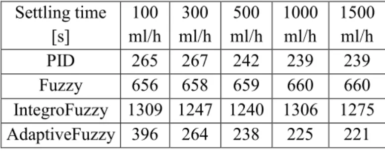
environment of the steady-state output [8]. (The ±1% range for control signal in steady-state was the result of other system requirements.) The results are summarized in Table I.
Settling time [s]
100 ml/h
300 ml/h
500 ml/h
1000 ml/h
1500 ml/h
PID 265 267 242 239 239
Fuzzy 656 658 659 660 660
IntegroFuzzy 1309 1247 1240 1306 1275 AdaptiveFuzzy 396 264 238 225 221
Table I. Settling Time
The integro-fuzzy logic has increased settling time compared both to the PID controller and the original fuzzy controller. Hence, it can be said that this controller is not suitable for control, further tuning is necessary to achieve an acceptable result. On the other hand the adaptive fuzzy controller has almost the same settling time as the PID controller. Over 300 ml/h is slightly faster, but at 100 ml/h it is slower. The results are acceptable, but faster settling would be recommended under 100 ml/h.
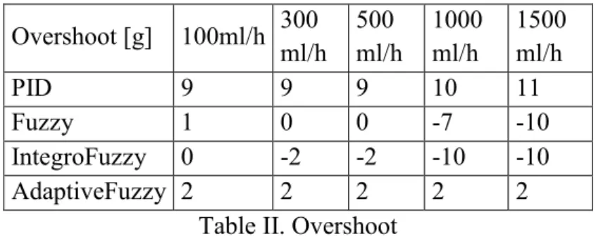
In order to examine the overshoot of the system, a worst case event was set: the pump segment was able to transfer 10% less fluid and at the beginning the system had 20 ml more transferred volume, than expected (-10% slope error, 20 ml offset error). The peak of the (first) overshoot was measured compared to zero error value. The measured overshoots are summarized in Table II.
17 Overshoot [g] 100ml/h 300
ml/h 500 ml/h
1000 ml/h
1500 ml/h
PID 9 9 9 10 11
Fuzzy 1 0 0 -7 -10
IntegroFuzzy 0 -2 -2 -10 -10
AdaptiveFuzzy 2 2 2 2 2
Table II. Overshoot
One advantage of the fuzzy controllers may be the small overshoot. The original fuzzy logic and the integro-fuzzy controller have minimal overshoot under 1000 ml/h, but over it they have as high overshoot as the PID controller has. The adaptive fuzzy controller has minimal overshoot independently of the flow.
The accuracy of the controllers was measured with the conditions used for measuring overshoot, but the measured quantity was calculated on a 200 seconds wide window after the steady-state was reached. The results of measurements are collected together in Table III.
Accuracy [g*s] 100 ml/h
300 ml/h
500 ml/h
1000 ml/h
1500 ml/h
PID 0 0 1 0 1
Fuzzy 494 -42 -718 -5721 -8504 IntegroFuzzy -662 -1823 -2322 -8214 -8573 AdaptiveFuzzy 135 48 16 -51 -84
Table III. Accuracy
The PID controller had no residual error and in steady state the volume of error slightly differed from 0. On the other hand the fuzzy controllers had residual error, which is clear from Table III. The size of the residual error depends on the flow and in the case of the original controller and the integro-fuzzy controller it is significant at almost any flow. (It has to be stated that the expectation would be the opposite. Still, the integro-fuzzy controller was unable for fine control and the small – 1 gram – errors were accumulated during the measurement. These are the causes for the difference.) The adaptive fuzzy controller has significantly smaller error in the steady state. If it is considered that these results were measured during 200 s, then it can be asserted, that the error of adaptive controller is sufficiently low. Furthermore, some trend can be seen in the case of adaptive logic, as if the integral of error was decreasing with the increase of flow. With simulations on the extremes (50 and 3000 ml/h) it was proved, that the error is sufficiently low even in this range (278 and -141 g*s respectively).
18
The quantitative measurement for robustness did not happen as it is hard to create quantitative requirements. However, the system stability was checked using errors out of the tolerance range [KJ3]. The swinging of the fluid bag was simulated by adding sinusoid signal on the output of the plant. The amplitude of the sine wave was chosen 10 ml, its frequency was set to 0.25 Hz. A considerably bad tube segment was simulated with a 30% slope error and with 100 ml offset error. The controllers’ performance was acceptable in every case.
Furthermore, the threshold for instability has not been reached.
At can be stated that, the integro-fuzzy controller showed significantly worse results, than the PID controller or the adaptive fuzzy logic. However, it has been shown that it is possible to control the system with the help of the integral of error.
The adaptive controller is almost as fast as the PID controller, and at higher flows it is even faster. It has minimal overshoot and the residual error is acceptable. As a result it can be said, that the adaptive fuzzy logic could substitute successfully the PID controller.
Furthermore, its adaptivity represents a huge benefit for embedded systems.
2.3.4. Evaluation in real environment
The designed controllers were not only tested, but the promising ones were also implemented in the real system. The PID controller was already tested. From the newly introduced controllers the adaptive fuzzy controller was implemented on a machine. The result of the measurement for this controller (at 500 ml/h fluid flow) is shown on Fig. 7.
7. Figure Result on target machine with adaptive fuzzy controller
It can be seen, that the real system is significantly slower, but according to [KJ1] this could be expected. The controller was able to compensate the 20 g error introduced, while the slope error was about 10%. Moreover, in the steady state, the system almost always had error, but it never left the ±1 g range. From the picture it can be seen that the resolution of the weighting scale can be measured to the error signal. This makes difficult to find the operating point
19
exactly. This way, it can be expected for the error to appear regularly which confirms the applicability of iterative learning control.
In spite of simulation results and real machine test it can be stated that either the classical PID controller or the adaptive fuzzy control is advised for implementation in a market product. The adaptive fuzzy controller has the advantage of not having any overshoot while the settling time is not increased. Furthermore, the adaptive fuzzy controller is capable to follow the changes of the operating point (changes of transfer volume of elastic tube segment). On the other hand, the PID controller is less demanding in term of computational capacity. Furthermore, the testing and tuning of the PID controller needs less skill and a- priori knowledge compared to the fuzzy controller. Altogether, it was demonstrated that in industrial environment the soft computing method can be as effective as the classical controller and it is only the choice of the company whether to utilize the benefits of the fuzzy controller or to stick the common solution.
2.4. Adaptive Neuro-Fuzzy Inference Systems
The amount of residual error raises the needs for other improved soft computing controllers.
Instead of complicating/redesigning the existing fuzzy controllers the applicability of adaptive neuro-fuzzy inference systems (ANFIS) was analyzed [35].
ANFIS systems use a layered structure as shown on Fig. 8. The task is to define the suitable membership functions for fuzzyfication and defuzzyfication (for the “if” and “then” parts) and to teach the rules for the decision making subsystem (in this case the parameters for the neurons) through training [36]. In order to check their efficiency and reliability two different ANFIS controllers were created.
8. Figure Internal structure of ANFIS [37]
In the first case a simple solution was applied; the controller contains an ANFIS system having the error signal as input, while its output is the control signal. In this solution 9 membership functions were used for the fuzzyfication and defuzzyfication (classical ANFIS - cANFIS). The distribution of membership functions followed the pattern used in the previous controllers: Trapezoid membership function are responsible for the extremities and
20
they reach up to ±200 grams where there is a safety threshold. The other membership functionS are triangle-shaped membership functions. Near zero the membership function is selected narrower and wider membership functions are used for bigger errors. Only adjacent membership function may intersect with each other.
2.4.1. Training sets
The training data contained a large recording. In this, the behavior of the PID controller was taken as a sample, and it was mimicked as it has most of the beneficial properties (except the presence of overshoot). Measurements were taken with the PID controller at flows of 100, 300, 500, 750, 1000 and 1500 ml/h [38]. At each flow the input and the output of the PID controller was recorded for:
no offset and no slope error,
±5g of offset error,
±1, ±3, ±5 and ±7% of slope error,
±10% of slope error and ±20g of offset error.
The records were concatenated, but some structures were cut off from them. At higher errors, it has appeared as if large control signal was necessary. In these cases, the rising part of the signal was cut off (e.g. in the case of 10% of slope error and -20g of offset error the first 15- 20 measurements were cut off, as this rising part was unnecessary and from the first part of the measurement were kept where the control signal did not changed namely, the compensation was executed). Overshoots were also cut off. This has resulted artificial signals with optimal behavior: The error signal is correlated to the control signal, without any overshoot.
As a result, the training data contained the expected behavior for high, middle and low flows and also for high, medium and low errors in various combinations. This training together with the above mentioned fuzzyfication and defuzzyfication functions has resulted a classical ANFIS controller which has replaced the controller of the system (as shown on Fig.2.).
2.4.2. Controller design
The other designed controller followed the structure of the adaptive fuzzy system from [KJ3]. However, in this case the fuzzy logic is replaced with an ANFIS. This resulted in the modified ANFIS (mANFIS) structure. The input (error signal) is integrated through an anti- windup system, and this is connected to the ANFIS. On the output of the ANFIS iterative learning control method is applied [39, 40, 41]; the saturated output value (control signal) is fed back through a memory unit (Fig. 9.).
21
9. Figure Modified ANFIS structure with ILC
The simplest description of an ILC can be described with the following equation [34]:
up+1 = up + K*ep (7),
where up is the input to the system during the pth repetition, ep is the control signal on pth repetition and K is a design parameter representing operations on ep. To implement it, a simple feedback loop was created, where the final saturated control signal is fed back through a memory unit. This means, that the K parameter is one and the output of the controller (ep) will affect the final control signal.
The ILC was introduced to eliminate the residual error, which was experienced in case of the classical ANFIS situation (cANFIS). Furthermore, a yet unmentioned problem occurred as well: In one hand the controller has to eliminate the inaccuracy of the tube segment caused by the production, while on the other hand the tube segment will fatigu over time. However, this fatigue will change very slowly (approx. 1-2% per day). As a result, the ILC was introduced to make the controller capable to follow this slow change [42].
The idea behind this concept was to combine the adaptivity reached through iterative learning control and the optimal control behavior reached by training sets. In this case 7 membership functions were used for fuzzyfication and defuzzyfication. The extremities were covered by trapezoid membership functions as characterized in Eq. (5) and the intermediate ones were triangle-shaped membership functions as described in Eq. (1). Near zero the membership functions were tighter, and only adjacent membership function were let to intersect each other [43].
Training data was manually generated in this case. The target values of the control signal were extracted from the measurements done with the PID controller (when there was only slope error). The output was defined to reach this limit in 10-20 steps (more steps in case of high flows, less steps in case of low flows). The goal was to avoid the remaining overshoot and achieve better result compared to the already mentioned PID controller.
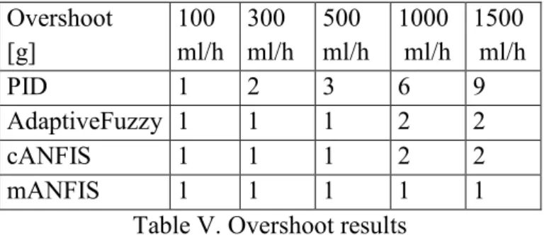
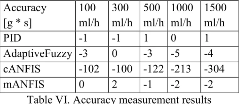
2.4.3. Evaluation of controller performance
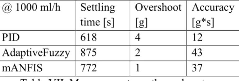
Results are presented mostly through the defined metrics just like above. The four controllers (PID as reference, adaptive fuzzy system as best solution from previous comparison, classical ANFIS, and modified ANFIS) were compared through the given properties and