Computers & Industrial Engineering

(1)

Contents lists available atScienceDirect

Computers & Industrial Engineering

journal homepage:www.elsevier.com/locate/caie

Risk-Based X-bar chart with variable sample size and sampling interval

Zsolt Tibor Kosztyán

^⁎

, Attila Imre Katona

Department of Quantitative Methods, University of Pannonia, Egyetem utca 10, Veszprém, Hungary

A R T I C L E I N F O

Keywords:

Adaptive control charts Measurement uncertainty Risk-based approach

A B S T R A C T

Flexibility is increasingly important in production management, and adaptive control charts (i.e., control charts with variable sample size and/or variable sampling interval) have significant importance in thefield of statistical process control. The value of the variable chart parameters depends on the detected process parameters. The process parameters need to be estimated based on observed values; however, these values are distorted by measurement uncertainty. Therefore, the performance of the method is strongly influenced by the precision of the measurement. This paper proposes a risk-based concept for the design of anX-bar chart with variable sample size and sampling interval. The optimal set of the parameters (control line, sample size and sampling interval) is determined using genetic algorithms and the Nelder-Mead direct search algorithm to minimize the risks arising from measurement uncertainty.

1. Introduction

For traditional control charts, afixed sample sizen,fixed sampling intervalhand width coefficient of control limitskare determined. The evolution of production processes resulted in the development of more flexible control charts, where the chart parameters change based on the characteristic of the monitored process. In this case, additional levels of the chart parameters are considered. If the process is said to be“in- control”, a smaller sample size, longer sampling interval and wider accepting interval are used. Conversely, in the case of an“out-of-control” process, a stricter control policy is applied (larger sample size, shorter sampling interval, and narrower accepting interval) (Lim, Khoo, Teoh, & Xie, 2015).

Reynolds, Amin, Arnold and Nachlas were theﬁrst scholars to develop anX-bar chart with variable sampling interval (VSI) (Reynolds, Amin, Arnold, & Nachlas, 1988), and this research inspired a number of researchers to design and improve VSI control charts (Bai & Lee, 1998;

Chen, 2004; Chew, Khoo, Teh, & Castagliola, 2015; Naderkhani &

Makis, 2016; Runger & Pignatiello, 1991).

Subsequently Prabhu, Runger and Keats developed anX-bar chart with adaptive sample size (VSS) (Prabhu, Runger, & Keats, 1993) and opened the way for research on VSS control charts (Chen, 2004; Costa, 1994; Tagaras, 1998).

As a further improvement, in VSSI control charts (variable sample size and sampling interval), the sample size and sampling interval are modiﬁed simultaneously (Chen, Hsieh, & Chang, 2007; Costa, 1997, 1998, 1999; De Magalhães, Costa, & Moura Neto, 2009). Numerous

studies apply economic designs to determine the optimal parameter set for these adaptive control charts to minimize the average cost during the control process (Chen, 2004; Chen et al., 2007; Lee, Torng, & Liao, 2012; Lin, Chou, & Lai, 2009).

Adaptive control charts have had increasing interest in the recent years. Some of the more recent approaches are Safe et al. which developed VSI EWMA control chart using Multi Objective Optimization (Safe, Kazemzadeh, & Gholipour Kanani, 2018), andYue and Liu (2017) which introduced a nonparametric EWMA chart using variable sampling interval. In another variant of the VSI control chart family, Yeong et al. designed EWMA-γ²chart in order to monitor the coeﬃcient of variation (Yeong, Khoo, Tham, Teoh, & Rahim, 2017). There have been new VSS control charts developed also in the recent years (see:Aslam, Arif, & Jun, 2016; Costa & Machado, 2016; Teoh, Chong, Khoo, Castagliola, & Yeong, 2017). Asﬁnal reference, we note that Salmasina et al. proposed a Hotelling’s T²chart with variable parameters with the integration of production planning and maintenance policy as well (Salmasnia, Kaveie, & Namdar, 2018).

1.1. Control charts and risk-based aspect

Producers’and suppliers’risks are frequently discussed topics in the field of conformity or process control (see e.g.:Lira, 1999). Risks can arise from different sources, such as uncertainty in the real process parameters or imprecision of the measuring device. The effect of parameter estimation on the performance of Shewhart control charts was analyzed in several studies (see:Jensen, Jones-Farmer, Champ, &

https://doi.org/10.1016/j.cie.2018.04.052

Received 7 November 2017; Received in revised form 26 April 2018; Accepted 27 April 2018

⁎Corresponding author.

E-mail addresses:kzst@gtk.uni-pannon.hu(Z.T. Kosztyán),akatona@gtk.uni-pannon.hu(A.I. Katona).

Available online 01 May 2018

T

(2)

Woodall, 2006). In addition, Zhou showed that parameter estimation has a signiﬁcant eﬀect on the in-control average time to signal (ATS) when using an adaptive VSSI X-bar chart. The study also developed an optimal design for the sample size (Zhou, 2017).

Not only uncertainty in the process parameters but also measurement uncertainty as risk factors can lead to serious consequences. If the measuring device or process is not suﬃciently accurate, incorrect decisions (such as unnecessary or missed maintenance) can be made during the control of the production process (Pendrill, 2008). Thus, the rate of the producer’s and customer’s risk is strongly dependent on the uncertainty in the measurement and can cause loss of prestige for a manufacturer company. In many cases, the eﬀect of measurement uncertainty is decreased by providing more accurate measuring devices or taking multiple samplesLinna and Woodall (2001). Nevertheless, it is common for the improvement of a measurement device or process to run into technological limitations and it is often impossible for multiple samples to be taken due to high sampling cost (e.g., destructive sampling). To address these problems, several adjustments must be made to the control process with consideration of measurement error.

Several studied aimed to analyze the effect of measurement error on statistical control charts. Mittag and Stemann showed that gauge imprecision can strongly affect the effective application of X-S control charts and the ability to detect process shifts (Mittag & Stemann, 1998).

Linna and Woodall proposed a measurement error model with covari- ates with the following form:

= + + ∊

Y A BX (1)

whereYis the observed value,Xis the real (true) value of the monitored product characteristic, AandB are constants (B>1) and∊is random error, which is independent ofX, assuming a normal distribution with mean 0 and varianceσ_m²(∊Ñ (0,σ_m²)) (Linna & Woodall, 2001).

They investigated how measurement error (based on the referred model) inﬂuences the performance ofX andS²charts. Several studies adopted this model and investigated the performance of diﬀerent types of control charts under the presence of measurement error while assuming linearly increasing variance (Haq, Brown, Moltchanova, & Al- Omari, 2015; Hu, Castagliola, Sun, & Khoo, 2015, 2016a; Maleki, Amiri, & Ghashghaei, 2016; Maravelakis, 2012; Maravelakis, Panaretos,

& Psarakis, 2004).

The impact of measurement error was considered in terms of not only the statistical but also the economical design of control charts.

Rahim investigated the eﬀect of non-normality and measurement error on the economic design of the ShewhartX chart (Rahlm, 1985). Yang extended the analysis to the asymmetricX andScharts.Yang (2002), and further studies proposed an economical design method for memory- based control charts, such as the exponentially weighted moving average (EWMA) chart based on measurement error (Abbasi, 2016;

Saghaei, Fatemi Ghomi, & Jaberi, 2014). Emphasizing the importance of the eﬀect of measurement error, several papers discussed its impact on process capability studies and proposed adjustments to improve the accuracy and reliability of the process performance indices (Baral &

Anisa, 2015; Grau, 2011; Pearn, Shu, & Hsu, 2005; Wu, 2011).

Kosztyán and Katona highlighted the importance of considering the measurement uncertainty related to the multivariate T² chart and proposed a method to reduce the risks during the control process (Kosztyán & Katona, 2016). Their method assigns cost values to the decision outcomes and applies a risk-based approach instead of the traditional approach in statistical process control (no consideration of measurement uncertainty during the control phase). When considering measurement uncertainty, there was an ̃4% decision cost reduction achieved by reducing type II errors. Although the risk-based multivariate control chart (RBT²) reduces the cost of decision outcomes, it applies onlyﬁxed parameters (i.e., sample size, sampling interval).

This study identiﬁes four types of decision outcomes:

•

correct acceptance

•

correct rejection

•

incorrect acceptance (type II error)

•

incorrect rejection (type I error)

The control line of a risk-based control chart is optimized to minimize the total cost arising from the four types of decision outcomes.

This method achieves better performance than that when using a re- commended coverage factor for the control limits.

The aim of this research is to improve the RB (risk-based) chart with variable parameters (sample size and sampling interval). The performance of the VSSI RB chart (risk-based control chart with variable sample size and sampling interval) is compared with that of the traditional control chart based on the following conditions:

1. Performance of the control chart when decision risks are not considered (kandware chosen andn h n₁, , ,₁ ₂ andh₂are optimized).

2. Performance of the control chart when the warning and control limits and the variable setup are optimized based on decision costs (using genetic algorithms).

3. Performance of the control chart with adjusted warning and control limits using a hybrid function to obtain more accurate results (with the Nelder-Mead direct search algorithm).

Although some studies have focused on the development of adaptive VSS (Hu, Castagliola, Sun, & Khoo, 2016b) and VSI control charts (Hu, Castagliola, Sun, & Khoo, 2016a) in the presence of measurement error, this paper aims to extend Kosztyán and Katona’s model with the joint consideration of variable sample size and sampling interval (VSSI).

1.2. Traditional VSSI control charts

Consider a process with observed values following a normal distribution with expected value μ and varianceσ². When a Shewhart control chart withﬁxed parameters is used, a random sample (n0) is taken every hour (denoted byh0). The observed statistic is plotted on the control chart, and the chart indicates when thei^thsample point falls outside the control limits determined asμ₀±kσ n₀, whereμ₀ is the center line, σ is the standard deviation of the process, andk is the control limit coeﬃcient:

= − LCL μ kσ

0 n

0 (2)

= +

UCL μ kσ

0 n

0 (3)

In the case of a VSSI control chart, the sample size and sampling interval vary between two levels. Theﬁrst level represents a parameter set with loose control (n h₁, ₁) with a smaller sample size and longer sampling interval, and the second level is a strict control policy (n h2, 2) with a larger sample size and shorter sampling interval. The parameters n and h must satisfy the following relations: n₁<n₀<n₂ and

< <

h₂ h₀ h₁, wheren₀is the sample size andh₀is the sampling interval of the FP control chart (control chart withfixed parameters). The switch rule between the parameter levels is based on a warning limit coeffi- cientw. Therefore, a central region and warning region can be specified (Chen et al., 2007):

=⎡

⎣⎢

− + ⎤

⎦⎥ I i μ wσ

n i

μ wσ n i ( )

( ),

1 0 0 ( )

(4) and

=⎡

⎣⎢

− − ⎤

⎦⎥ ∪⎡

⎣⎢

+ + ⎤

⎦⎥ I i μ kσ

n i μ wσ

n i

μ wσ n i

μ kσ ( ) n i

( ),

( ) ( ) ,

2 0 0 0 0 ( )

(5)

= ∪

I i3( ) I1 I2 (6)

(3)

wherei=1,2…is the sample number,I₁denotes the central region, and I2the warning region. Let us assume that anX-bar chart is applied and thatx_idenotes the mean of thei^thsample. During the control process, the following decisions can be made (Lim et al., 2015):

1. Ifxi∈I1, the manufacturing process is in an“in-control”state and sample sizen₁and sampling intervalh₁are used to computex_i+₁. 2. If x_i∈I₂, the monitored process is “in-control”but x_i falls in the

warning region; thus,n2andh₂are used for the(i+1)^thsample.

3. Ifx_i ∉ I₁andx_i ∉ I₂, the process is out of control, and corrective actions must be taken. After the corrective action,x_i+₁falls into the central region, but there is no previous sample to determinen i( +1) and h i( +1). Therefore, as Prabhu, Montgomery, and Runger (1994)andCosta (1994)proposed, the next sample size and interval are selected randomly with probability p₀. p₀ denotes the probability that the sample mean falls within the central region. Simi- larly,1−p₀ is the probability that the sample point falls within the warning region.

VSSI control charts are a powerful tool to control manufacturing processes. However, VSSI control charts do not consider measurement uncertainty (and the risk of the decisions) as part of the control limit calculation. Due to the distortion of the measurement error, the“in- control”and“out-of-control”statements and even the switching decision between( , )n h1 1 and( , )n h2 2 can be incorrect.

2. The decision costs

Measurement uncertainty can lead to incorrect decisions during the control of a manufacturing process. Based on the model ofKosztyán and Katona (2016), the decision outcomes can be extended for a VSSI chart as follows (seeFig. 1):

Table 1shows the possible decision outcomes when a VSSI control chart is applied. Due to the distortion eﬀect of the measurement uncertainty, the real product characteristic can diﬀer from the observed product characteristic, resulting in incorrect decisions. InTable 1,“in (CL)”and“out(CL)”denote the in-control and out-of-control statements based on the control line(s), and“in(WL)”and“out(WL)”represent the sample location relative to the warning limits. In addition,xis the real product characteristic, andyis the detected one.I₁,I₂andI₃denote the regions according to Eqs. (2)–(4). If the detected characteristic falls within the out-of-control region based on the control line, it excludes the potential of being “in-control” based on the warning limit.

Similarly, if the real product characteristic is out-of-control (based on the control lines), the sample point cannot fall within the central region. These cases are represented by a black cross in the table. Each case can be described as follows (the number of each case is represented by number in the right left corner of each cell in the table):

•

Case 1: Both the detected and the real product characteristic fall within the central region. The decision is a correct acceptance.

•

Case 2: The detected characteristic is in the warning region but the real characteristic is in the central region. In this case, the sample size is increased and the sampling interval is reduced. However, these changes are unnecessary, and the decision is incorrect.

•

Case 3: The process is out-of-control based on the detected product characteristic, but the real characteristic falls within the central region. The expected value of the process is in-control, but a shift is detected incorrectly. Therefore, an unnecessary corrective action is taken (type I error).

•

Case 4: The real characteristic is within warning region (out-of- control based on the warning limit) but an in-control statement is detected. In this case, the sample size should be increased and the sampling interval should be reduced; however, this action is not taken. This failure reduces the performance of the VSSI chart because it increases the time for detection and correction.

in (WL) out (WL) in (WL) out (WL)

x I

1

x I

1

x I

1

and and and

y I

1 (1)

y I

2 (2)

y I

3 (3)

x I

2

x I

2

x I

2

and and and

y I

_{1 (4)}

y I

_{2 (5)}

y I

_{3 (6)}

x I

3

x I

3

x I

3

and and and

y I

_{1 (7)}

y I

_{2 (8)}

y I

_{3 (9)}

Detected product characteristic

in (CL) out (CL)

in (WL)

out (WL)

in (WL)

out (WL) in (CL)

out (CL) Real

Fig. 1.The structure of decision outcomes.

Table 1

Elements of the cost of decision outcomes.

Sign Name

n Sample size

Nh Produced quantity in the considered interval (h)

cp Production cost

cmf Fixed cost of measuring

cmp Proportional cost of measuring

cc Cost of qualiﬁcation

cs Cost of switching

d1 Weight parameter for switching

ci Cost of intervention

d2 Weight parameter for intervention

cr Cost of root cause search

cid Cost of delayed detection

c_f Cost of false alarm identiﬁcation

cmi Cost of missed intervention

cr Cost of restart

cma Maintenance cost

(4)

•

Case 5: Both the detected and real characteristics fall within the warning region. The sample size is increased, the sampling interval is reduced, and the decision is correct.

•

Case 6: Out-of-control is detected; however, the real characteristic falls within the warning region. Corrective action is taken, but the switch between the chart parameters ( , )n h would be suﬃcient.

Therefore, the decision is incorrect.

•

Case 7: In-control state is detected andyis located in the central region, but the process is out-of-control. The decision is incorrect, and corrective action is not taken, which is a type II error.

•

Case 8: Similar to Case 7, butyis in the warning region. Therefore, this case is more positive than Case 7 because a strict control policy is applied. Thus, a shorter time is needed to identify the process shift.

•

Case 9: The real and detected product characteristics are out-of- control; therefore, the decision is correct.

For clariﬁcation, Fig. 2 shows an example of the nine decision outcomes described above.

2.1. Speciﬁcation of decision costs

During process control, several decisions can be made. In this subsection, we introduce the cost structure of each decision outcome. First, the elements of the decision outcomes must be speciﬁed.

Table 1shows the speciﬁed cost components in the cost structure.

The following costs are involved in each decision:

•

expected total production cost

•

cost of measuring

•

cost of qualiﬁcation

cpdenotes the proportional production cost, andNhis the expected number of manufactured products in interval h(where his the time interval between two samples). Therefore, the expected total production cost can be estimated as N ch p. The cost of measurement can be divided into two parts, afixed cost (cmf) and a proportional cost (c_mp) depending on sample size (n). Thefixed measurement cost (e.g., labor, lighting, operational cost of the measurement device) arises in every measurement irrespective ofn.cmpis the expected measurement cost for a sample that strongly depends on sample size (especially significant for destructive measurement processes). Thus, the expected total measurement cost can be estimated asncmp+cmf. In addition, the cost of qualificationc_q must be considered (charting, plotting, labor). Since

+ + +

N c_{h p} nc_mp c_mf c_q is a part of each cost component, we apply a constantN ch p+ncmp+cmf +cq=c0for simplicity.

Some cost components arise in only special cases. The cost of switchingc_sis the cost of the modiﬁcation of the VSSI chart parameters

(n h, ).cidenotes the cost of intervention, including the cost of the machine stop and root cause search. If the root cause cannot be identiﬁed, it is likely that a false alarm occurred. In this case, the cost of maintenance (cma) cannot be speciﬁed. On the other hand, this cost component must be considered when a root cause is found and the machine must be maintained (e.g., cost of the parts, labor cost).

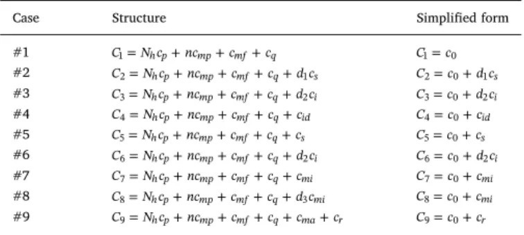
The weighting parameters must also be specified. Some cases (e.g., Case 2 and Case 5) are similar but have different estimated costs. This difference can be derived from the necessity of the decision. For example, in Cases 2 and 5, the detected characteristic is located in the warning region but the decision is necessary in Case 2 and unnecessary in Case 5. In similar cases, the unnecessary decision must be multiplied by the weighting parameter to consider the surplus modifications during control. Therefore,d₁is the weighting parameter for the cost of unnecessary switching, and d₂ is the weighting parameter for unnecessary intervention.Table 2includes the forms of the decision costs assigned to the decision outcomes.

During the control process, suﬃcient cost must be assigned to each sampling point. The assigned costs must be further aggregated to determine the total decision cost from theﬁrst sample to the actual one.

The goal is to set the optimal value of the coverage factork(and the optimal values of the control linesUCL LCL, ) and the optimal parameter set for the switching (n h, ) to minimize the total decision cost. A detailed introduction for this optimization method is provided in Section3.

3. The RB VSSIX-bar chart

3.1. Overview of the proposed chart construction method

In this subsection, the authors introduce the construction process of the RB VSSIX-bar chart, which can be summarized as follows:

1. Calculation of the traditional control chart parameters (as initial values for the optimization).

Fig. 2.Demonstration of the nine decision outcomes on a control chart.

Table 2

Elements of the costs of the decision outcomes.

Case Structure Simpliﬁed form

#1 C1=N ch p+ncmp+cmf+cq C1=c0

#2 C2=N ch p+ncmp+cmf+cq+d c1s C2=c0+d c1s

#3 C3=N ch p+ncmp+cmf+cq+d c2i C3=c0+d c2i

#4 C4=N ch p+ncmp+cmf+cq+cid C4=c0+cid

#5 C5=N ch p+ncmp+cmf+cq+cs C5=c0+cs

#6 C6=N ch p+ncmp+cmf+cq+d c2i C6=c0+d c2i

#7 C7=N ch p+ncmp+cmf+cq+cmi C7=c0+cmi

#8 C8=N ch p+ncmp+cmf+cq+d c3mi C8=c0+cmi

#9 C9=N ch p+ncmp+cmf+cq+cma+cr C9=c0+cr

(5)

2. Estimation of the cost components described in Section2.

3. Calculation of the overall decision cost considering the initial (traditional) control chart parameters.

4. Optimization of the control chart parameters via simulation.

(a) Control chart parameter optimization via genetic algorithm.

(b) Improvement of the optimization result using the Nelder-Mead direct search method.

In the following, we describe the above steps in detail.

Step 1:

The control lines of the traditionalX-bar chart can be computed with(2) and (3). The VSSI RBX-bar chart uses these control lines as initial values. During optimization, the optimal values ofUCLandLCL that minimize the total decision cost are determined by simulation.

Step 2:

The cost values for each case (C C1, 2,…C9) must be estimated. This can be supported by an ERP system, where the estimated costs can be queried from a control module. Otherwise, each cost component should be estimated by experts. Each cost must be assigned to the suitable case (according toTable 1) to calculate the total decision cost during the simulation (or during the control process).

Step 3:

The number of occurrences each case must be quantiﬁed and multiplied by the assigned cost value. In the cost structure,

+ + +

N ch p ncmp cmf cqis the cost component that arises in every case;

therefore, to simplify the formula, it is replaced withC_c.

∑

⁼ ⁺ ⁺ ⁺ ⁺ ⁺ ⁺ ⁺ ⁺

+ + + + + +

+ + +

C q C q C d c q C d c q C c q C c

q C d c q C c q C d c

q C c c

( ) ( ) ( ) ( )

( ) ( ) ( )

( )

c c s c i c id c s

c i c mi c mi

c ma r

1 2 1 3 2 4 5

6 2 7 8 3

9 (7)

whereq q₁, ₂…q₉ are the numbers of time each case occurs during the simulation and ∑C is the total decision cost. The equation can be simpliﬁed using the cost values of each decision outcome:

∑

^C⁼^{q C}1 1⁺^{q C}2 2⁺^{q C}3 3⁺^{q C}4 4⁺^{q C}5 5⁺^{q C}6 6⁺^{q C}7 7⁺^{q C}8 8⁺^{q C}9 9

(8) Step 4:

The coverage factorkand the variable parameters( , , , , )n n h h w₁ ₂ ₁ ₂ are optimized to minimize the value of∑C. Two approaches are used to optimize the chart parameters. The integer parameters,( , , , )n n h h1 2 1 2 are optimized using genetic algorithms as theﬁrst step. In the second step, the Nelder-Mead algorithm is used as a hybrid function. This approach optimizes the continuous parameters( , )k w to obtain more precise results for the modiﬁed warning and control limits.

3.2. Simulation of the control procedure and optimization

As theﬁrst step, ann×mmatrix (denoted byX) of the“real”values is generated with expected value μ_x and standard deviation σ_x. Similarly, ann×mmatrixE, representing the measurement error, is also generated. We use Matlab’s“pearsrnd”function to generate the measurement error matrix. This function returns ann×m matrix of random numbers according to the distribution in a Pearson system.

With this approach, the four parameters (expected value, standard deviation, skewness and kurtosis) of the measurement error distribution can be easily modiﬁed.

After these two matrices are generated, the matrix of “observed”

values can be estimated in the following manner:

=A+B +

Y X E (9)

whereYis ann×mmatrix containing the estimated observed values.

In bothXandY, each row represents a possible sampling event and each element in a row represents all the possible products that can be selected for sampling. To construct the VSSIX-bar chart, the VSSI rules must be applied toXandY. The algorithm loops through the matrices

from theﬁrst row to then^throw.

Letx̂be the vector of sample means fromX, and letŷbe the vector of sample means selected fromY. If thei^thsample mean (with sample sizen₁) falls within the warning region,n₂andh₂must be used in the next sampling:

a. Ifxĵ∈I2, then thei+h₂^throw fromXis selected for sampling and elementn₂is selected randomly from thei+h₂^throw. Otherwise, the

+

i h₁^throw is selected with sample sizen₁.

b. Ify_ĵ∈I2, then thei+h₂^throw fromYis selected for sampling and elementn2is selected randomly from thei+h₂^throw. Otherwise, the

+

i h₁^throw is selected with sample sizen1.

In the next step, each element inx̂andŷis compared and assigned to a decision outcome described in Section2. In theﬁnal step of the simulation, the total decision cost is calculated as the summation of the cost of each decision.

We use genetic algorithms tofind the optimal set of integer design parameters (n n h h₁, , ,₂ ₁ ₂) that minimizes the total cost function given by Eq.(8). This approach imitates the principles of natural selection and can be applied to estimate the optimal design parameters for statistical control charts. In thefirst step, this method generates an initial set of feasible solutions and evaluates them based on afitness function. In the next step, the algorithm:

(1) selects parents from the population;

(2) creates crossover from the parents;

(3) performs mutation on the population given by the crossover; op- erator

(4) evaluates theﬁtness value of the population.

This steps are repeated until the algorithmﬁnds the bestﬁtting solution (Chen et al., 2007). Then, the Nelder-Mead method is applied as a hybrid function to search for the optimal values of the continuous variables (w k, ).

This is a two-dimensional case, where the algorithm generates a sequence of triangles converging to the optimal solution. The objective function isC n n h h w k( , , , , , )1 2 1 2 , wherewis the warning limit coeﬃcient andkis the control limit coeﬃcient. Note that the other design parameters (n n h h1, , ,2 1 2) are already optimized by genetic algorithms; therefore, in this step, we use the objective functionC w k( , ), where0<w<k andw k, ∈.

In the two-dimensional case, three vertices must be determined, and the cost function is evaluated for each vertex. In theﬁrst step, ordering is performed on the vertices:

Ordering:

The vertices must be ordered based on the evaluated values of the cost function:

< <

C w kB( 1 1, ) CG(w k2 2, ) CW(w k3, )3 (10) whereCBis the best vertex with the lowest total cost,CG(good) is the second-best solution andCWis the worst solution (with the highest cost value). Furthermore, letv₁=(w k_{1 1}, ),v₂=(w k_{2 2}, )andv₃=(w k₃, )₃ denote the vectors of each point.

The approach applies four operations: reﬂection, expansion, contraction and shrinking.

Reﬂection:

The reﬂection point is calculated as:

=

= ⎡

⎣⎢

+ + ⎛

⎝

+ − ⎞

⎠

+ + ⎛

⎝

+ − ⎞

⎠

⎤

⎦⎥

= +

+ ⎛

⎝

+ − ⎞

⎠ v w k

w w

α w w

w k k

α k k k

α v

v v v

v [ , ]

2 2 ,

2 2

R R RT

T

1 2 1 2

3 1 2 1 2

3

1 2 1 2

3 (11)

where v_R is a vector denoting the reﬂection point, w kR, R are the

(6)

coordinates of the reﬂection point andα>1is the reﬂection parameter.

C w kR( R, )R must be evaluated, and v3 needs to be replaced with vR if

⩽ <

C w k_B( _{1 1}, ) C w k_R( _R, )_R C_G(w k_{2 2}, ). Expansion:

After reﬂection, expansion is performed ifC w kR( R, )R <C w kB( B, )B:

=

= ⎡

⎣⎢

+ + ⎛

⎝ − + ⎞

⎠

+ + ⎛

⎝ − + ⎞

⎠

⎤

⎦⎥

= +

+ ⎛

⎝ − + ⎞

⎠ w k

w w

β w w w k k

β k k k

β v

v v

v v v

[ , ]

2 2 ,

2 2

E E E T

R R

T

R

1 2 1 2 1 2 1 2

1 2 1 2

(12) wherev_Edenotes the reﬂection point with coordinatesw_Eandk_Eandβ is the expansion parameter.C w kE( E, E)is evaluated andv₃ is replaced withvEifC w kE( E,E)⩽C w kR( R, )R.

Contraction:

Outside contraction is performed if C_G

⩽ <

w k C w k C w k ( 2 2, ) R( R, )R W( 3, )3:

=

= ⎡

⎣⎢

+ + ⎛

⎝ − + ⎞

⎠

+ + ⎛

⎝ − + ⎞

⎠

⎤

⎦⎥

= +

+ ⎛

⎝ − +

⎞

⎠ w k

w w

γ w w w k k

γ k k k

γ v

v v

v v v

[ , ]

2 2 ,

2 2

OC OC OCT

R R

T

R

1 2 1 2 1 2 1 2

1 2 1 2

(13) Here,v_OC is the point that can be derived by outside contraction with coordinates wOC andkOC; furthermore, 0<γ<1 is the contraction parameter. Then, evaluateC_OC(w_OC,k_OC). IfC_OC(w_OC,k_OC)⩽C w k_R( _R, )_R, replace v₃with v_OC; otherwise, the shrinking operation must be performed.

The inside contraction point denoted by vIC is computed if

⩾

C w k_R( _R, )_R C_W(w k₃, )₃:

=

= ⎡

⎣⎢

+ − ⎛

⎝ − + ⎞

⎠

+ − ⎛

⎝ − + ⎞

⎠

⎤

⎦⎥

= +

− ⎛⎝ − + ⎞

⎠ w k

w w

γ w w w k k

γ k k k

γ v

v v

v v v

[ , ]

2 2 ,

2 2

IC IC ICT

R R

T

R

1 2 1 2 1 2 1 2

1 2 1 2

(14) In this case,CIC(wIC,kIC) is evaluated, and the point with the highest total decision cost v₃ is replaced with vIC; otherwise, the shrinking operation is used.

Shrinking:

Shrinking must be performed for then^thandn+1^thpoints. Since we consider the two-dimensional case of the design parameterswandk, this operation is performed forv2andv3:

= w k = w +δ w−w k +δ k−k = +δ − v₂_S [ ₂_S, ₂_S]^T [ ₁ ( ₂ ₁),₁ (₂ ₁)]^T v₁ (v₂ v₁)

(15)

= w k = w +δ w−w k +δ k−k = +δ − v3S [ 3S, 3S]^T [ 1 ( 3 1),1 (3 1)]^T v1 (v3 v1)

(16) wherev2S andv3S are the shrunk points derived from v2 andv3, re- spectively (Fan, Liang, & Zahara, 2006).

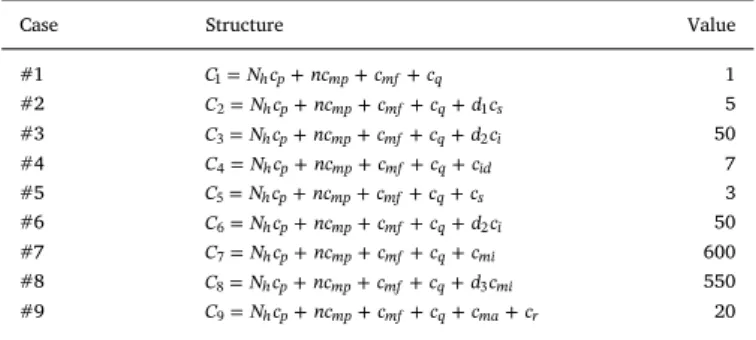
4. Practical example

In this section, we demonstrate the applicability of the proposed method with a practical example.Table 3shows the cost of the nine decision outcomes as input parameters.

Furthermore, the production process follows a normal distribution with expected value μ_x=100 and standard deviation σx=0.2. The measurement error has a normal distribution with expected value

=

μ_m 0 and standard deviationσ_m=0.02. In theﬁrst step,k=3and

=

w 2 are used to calculate the control and warning limits (kis the control limit coeﬃcient anwis the warning limit coeﬃcient). The other design parameters (n n h h1, , ,2 1 2) are optimized to minimize the total cost

of the decisions, as described by Eq.(8). Next, the design parametersk andware optimized using the Nelder-Mead direct search method. In this study,k^∗andw^∗denote the optimal values ofkanw.Fig. 3shows the value of the objective function in each iteration of the optimization.

InFig. 3, the circles represent the actual values of the objective function when the genetic algorithm is running. Similarly, the triangles show the objective function values during the Nelder-Mead approach.

The Nelder-Mead method achieves an additional 0.5% cost reduction, but more importantly, the results derived from the hybrid function are more stable.

Table 4shows the results of the proposed method.

The total cost of decisions is reduced by 13.5% when applying the proposed method. The integer parameters( , , , )n n h h1 2 1 2 are optimized in the initial state to minimize the total cost of decisions.

Kosztyán et al. proposed a risk-based approach for conformity control (Kosztyán, Hegedűs, & Katona, 2017), and another study developed a risk-based multivariate T²chart (Kosztyán & Katona, 2016).

Both approaches achieved an approximately 2–4% reduction in the total decision cost. However, as the previous example shows, the VSSI X-bar chart outperforms the traditionalX-bar chart, and the proposed method reduced the total decision cost by 13.5%. To explain the out- standing reduction rate, inFig. 4, we highlight an interval from the time series of the controlled product characteristic to compare the behavior and patterns of the risk-based and traditional VSSIX-bar charts.

The traditional control chart is shown in the upper-left corner of Fig. 4, where the control and warning lines were set to their initial values (measurement uncertainty was not considered), X denotes the sample mean of the real (simulated) product characteristic, andY denotes the sample mean of the observed product characteristic (simulated measurement error is added toX). The bar chart in the lower-left corner shows the cost value assigned to each decision (to each plot of the time series). Similarly, the right side of the chart shows the pattern if the risk-based VSSIX-bar chart is used and the control and warning limits are optimized while taking the measurement uncertainty into account.

In the case of the adaptive control chart, the pattern of the control chart depends not only on the values of the control limits but also on the width of the warning interval. The sample size and sampling interval are determined by the position of the observed sample mean and warning limits. Therefore, the distorting eﬀect of the measurement error can create very diﬀerent scenarios based on the control chart patterns. If the observed sample mean falls within the warning region and the real sample mean is located within the acceptance interval, the sample number will be increased and the sampling interval will be reduced incorrectly, leading to increased sampling costs. In the opposite case, sampling will be skipped, which will delay the detection of the process mean shift.

As shown inFig. 4, when the traditional VSSI chart is applied, the two process patterns (observed and real) become separated from each other by the7^thsampling. A diﬀerent sampling policy will then be used due to the eﬀect of the measurement uncertainty, causing separation of Table 3

Elements of the cost of the decision outcomes.

Case Structure Value

#1 C1=N ch p+ncmp+cmf+cq 1

#2 C2=N ch p+ncmp+cmf+cq+d c1s 5

#3 C3=N ch p+ncmp+cmf+cq+d c2i 50

#4 C4=N ch p+ncmp+cmf+cq+cid 7

#5 C5=N ch p+ncmp+cmf+cq+cs 3

#6 C6=N ch p+ncmp+cmf+cq+d c2i 50

#7 C7=N ch p+ncmp+cmf+cq+cmi 600

#8 C8=N ch p+ncmp+cmf+cq+d c3mi 550

#9 C9=N ch p+ncmp+cmf+cq+cma+cr 20

(7)

the two control chart patterns. The sifted pattern continues until the point, where the two control policy is the same again. On the other hand, the risk-based VSSIX-bar chart takes measurement uncertainty into account and modiﬁes the warning interval, enabling betterﬁtting of the two control chart patterns. The shifted interval is denoted by the dark columns on the bar charts. The charts show that the RB VSSI chart reduces the length of the interval. Therefore, it reduces not only the decision costs due to the out-of control state but also decreases the number of incorrect decisions in the in-control state and compensates for the separation of the chart patterns. Therefore, a greater decision- cost reduction can be achieved with the VSSI chart compared to the Fig. 3.Convergence to the optimal solution with Genetic Algorithm and Nelder-Mead direct search.

Table 4

Performance of the proposed control chart.

n1 n2 h1 h2 k∗ w^∗ ∑C Δ (%)C

Initial state 2 4 2 1 3.00 2.00 1.236E+06 −

Optimization: GA 2 4 2 1 2.298 2.287 1.075E+06 −13.0 Optimization: GA + NM 2 4 2 1 2.298 2.175 1.070E+06 −13.5

Fig. 4.Comparison traditional and RB VSSI control chart patterns.

(8)

results of the referenced studies.

As a signiﬁcant contribution, this paper also raises awareness of the importance of considering measurement uncertainty in the ﬁeld of adaptive control charts.

In the practical example, the authors applied theY=A+BX+ε model of measurement error under the assumption of constant variance (A=0 andB=1). To investigate how the proposed model performs under linearly increasing variance, an additional simulation was con- ducted.Fig. 5shows the results of the simulation.

We used the same cost components as described inTable 3, but parametersAandBin the measurement error equation were changed in each iteration. The z-axis shows the achievable cost reduction rate ex- pressed as a percentage (Δ %C ) for each combination ofAandB. The blue dots show the raw results of the simulation, and a smoothed pane wasfitted to the data points to better illustrate the pattern. The results show that the proposed method still reduces the overall decision cost under linearly increasing measurement error variance; however, the model is sensitive to changes in parameterA(changes in parameterB do not significantly alter the cost reduction). If A> 0, the distance between XandYincreases significantly, indicating shorter sampling intervals and larger sample sizes. Although the proposed method achieves lower overall decision cost through modification of the warning and control limits, the increased cost from sampling increases the overall decision cost, limiting the cost reduction for the method.

Nevertheless, an approximately 4% cost reduction was achieved under linearly increasing variance due to the optimization of the control and warning limits.

5. Sensitivity analysis

Section4demonstrated the applicability of the method for the given example. The purpose of this section is to investigate the more general behavior (pattern) of the control chart parameters. Therefore, we analyze how changes in the cost components, standard deviation of the measurement error and skewness of the measurement error impact the value ofk^∗andw^∗. These factors are selected to assess the limitations of the proposed method. The kurtosis of the measurement error could also

be examined, but its impact was previously analyzed by Kosztyán et al.

The cost of type II errors is analyzedﬁrst.

5.1. Sensitivity analysis with respect to the cost of type II error

The 9 decision outcomes defined in this study must be assigned to different groups for a better understanding of the effects during the sensitivity analysis.

Therefore, we distinguish three groups of decision outcomes:

•

Group 1: Type I error decision outcomes, where the decision is incorrect due to an unnecessary action. Outcomes: #2, #3, #6.

•

Group 2: Type II error decision outcomes, where the decision is incorrect due to a missed action. Outcomes: #4, #7, #8.

•

Group X: The remaining decision outcomes, including the correct decisions. Outcomes: #1, #5, #9.

During the sensitivity analysis, each cost in Group 2 is multiplied by a changing coeﬃcient (a). Thus, thei^thcost is calculated as:

=

C4i a Ci· 4initial (17)

=

C₇_i a C_i· ₇_initial (18)

=

C₈_i a C_i· ₈_initial (19)

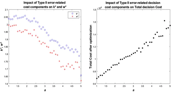
whereC₄_initial_{, 7}C_initial,and C₈_initialare the initial values of the decision costs related to cases #4, #7, and #8.a_iis the value of the coeﬃcient in the i^thrun within the simulation, andi=1,2,3…n i, ∈wherenis the total number of runs.Fig. 6shows the optimal values ofkandw(denoted by k∗andw^∗) as a function of the cost-changing coeﬃcienta.

InFig. 6, the circles represent the values ofk^∗and the crosses in- dicate the values ofw^∗. WhileC C4, 7andC8increase, the optimal values of bothkandwdecrease. If the cost of type II error decisions increases, the control policy will be stricter. Therefore, the control and warning limits must be moved closer to the central line of the control chart to avoid type II errors. An increase in type II-related costs does not have a signiﬁcant impact on the interval betweenk^∗andw^∗. Asaincreases, the Fig. 5.The cost reduction rate as a function of A and B.

(9)

control and warning limits move in the same direction simultaneously.

The impact of the type II error-related cost components on the overall decision cost was also investigated. As the results on the right side of Fig. 6show, the overall decision cost increases linearly with parameter a. Note that the analysis shows the overall decision cost after optimization. Although this method reduces the risk, the overall decision cost is higher if the consequences of type II errors are more serious.

To further analyze the behavior of the warning interval, we con- ducted a sensitivity analysis based on the sampling cost because it di- rectly inﬂuences the warning limit coeﬃcient.Fig. 7shows the results of the analysis.

Fig. 7shows the distance betweenk^∗andw^∗(k^∗−w^∗) as a function of the sampling cost (c_s). The higher the cost of sampling is, the greater the distance between the two limits. A higher sampling cost increases the warning limit coeﬃcient because the control is too expensive due to the frequently increased sample size and sampling interval. A lower sampling cost allows a stricter control policy for the warning limit.

5.2. Sensitivity analysis based on the standard deviation of the measurement error

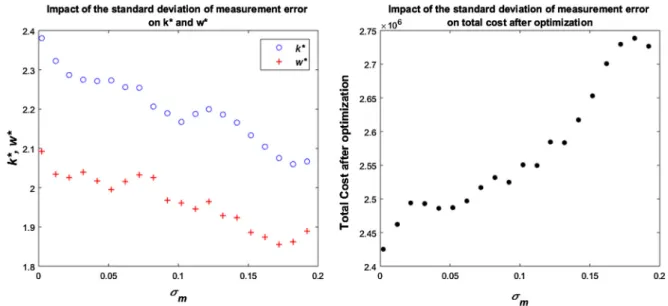
The behavior of the control limits was also examined while changing the standard deviation in the simulation. All the distribution parameters were held constant during the simulation except the standard deviation of the measurement error (σm).

AsFig. 8shows, the control limit coefficients (w^∗andk^∗) decrease as the standard deviation of the measurement error increases. A higher standard deviation (according to the measurement error) represents a stricter control policy; thus,w^∗andk^∗decrease. In this case, the effect of measurement uncertainty is increasingly significant; therefore, the approach reduces the length of the control interval to avoid type II errors. The distance between the two limits is nearly constant because the sampling cost does not change during the simulation. Nevertheless, the sampling cost has a significant impact on the distance betweenw^∗ ank^∗, as shown in the previous subsection. The results show thatσm

signiﬁcantly aﬀects the overall decision cost. A higher standard deviation of the measurement error results in a higher frequency of control measures, causing higher costs.

5.3. Sensitivity analysis base on the skewness of the measurement error Since Kosztyán et al. proved that the kurtosis of the measurement error distribution does not impact the control line value, we focus on the skewness of the measurement error distribution only.

In the simulation, the model parameters were the same, but the skewness of the measurement error distribution (denoted byγ) was modiﬁed in each iteration (starting with−1 and ending with 1).

Fig. 9shows the results of the sensitivity analysis.

In the simulation,k^∗andw^∗are not aﬀected by changes inγbecause sampling adjusts the skewed distribution to normal. Based on the central limit theorem, the average of the aggregated sample groups tend to normal (and the skewness will be more closer to 0). An illustrative example from the simulation is shown in the appendix inFig. 10.

This phenomenon is also reﬂected by the results related to the overall decision cost. Due to the central limit theorem, neither the limit coeﬃcientsk^∗andw^∗nor the overall decision cost react to changes in the skewness of the measurement error distribution.

In this section, the model sensitivity was analyzed from diﬀerent Fig. 6.Sensitivity analysis regarding type II error-related cost components.

Fig. 7.The width of warning interval as a function of sampling cost.

(10)

aspects; however, we note that uncertainty related to the process parameter estimation can also aﬀect the control chart parameters (Zhou, 2017). This paper focuses on the eﬀect of measurement uncertainty and proposes a method to develop a risk-based adaptive control charts. Nevertheless, the method can be extended to consider the process parameter estimation.

6. Summary and conclusion

This paper extends the consideration of measurement uncertainty to the ﬁeld of adaptive control charts. The proposed method not only optimizes the chart parameters (n n h h k w₁, , , , ,₂ ₁ ₂ ) but also adjusts the control and warning limit coeﬃcients (k^∗, andw^∗) to minimize the aggregated cost derived from the decision outcomes. Genetic algorithm and the Nelder-Mead method (as a hybrid function) are used during the chart-parameter optimization. A practical example is provided to demonstrate the features of the proposed method. With the assumed in- puts, the proposed method reduces the total decision cost by13.5%

compared to the“traditional”VSSIX-bar chart (due to the reduction of incorrect decisions). Several sensitivity analyses are also provided to

assess the behavior of the optimized parametersk w^∗, ^∗and the overall decision cost (providing more general conclusions compared to those from the practical example).

The contribution of the proposed method can be defined from two aspects. As an academic contribution, this study extends the dimension of the decision matrix defining decision outcomes regarding the warning limits as well. In addition the results showed that measurement uncertainty can be described by thefirst two moments of its distribution function (expected value and standard deviation) when the RB VSSI chart is applied because the result of the optimization is not sensitive to the skewness of the distribution. From decision maker’s point of view, the results show that consideration of measurement uncertainty is important not only from control lines’ perspective but decision costs can be significantly reduced in the in-control state by adjusting the warning limits. Therefore, this article shows that the risk-based approach can be used effectively in the field of adaptive control charts.

Previous studies (Kosztyán et al., 2017; Kosztyán & Katona, 2016) showed that the risk-based approach can be used in diﬀerentﬁelds of quality control (conformity control, multivariate control chart). This Fig. 8.Sensitivity analysis regarding standard deviation of measurement error.

Fig. 9.Sensitivity analysis regarding the skewness of measurement error distribution.

Computers & Industrial Engineering