Analysis and Control of Quasi-Polynomial DAE Systems
Ph.D. Thesis
Barna Pongrácz
Supervisor: Professor Katalin Hangos Consultant: Gábor Szederkényi, PhD
Information Science PhD School Department of Computer Science
University of Pannonia Veszprém, Hungary
Process Control Research Group
Computer and Automation Research Institute Hungarian Academy of Sciences
Budapest, Hungary
2008
Analysis and Control of Quasi-Polynomial DAE Systems
Értekezés doktori (PhD) fokozat elnyerése érdekében Írta:
Pongrácz Barna
Készült a Pannon Egyetem Informatikai Tudományok Doktori Iskolája keretében Témavezető: Dr. Hangos Katalin
Elfogadásra javaslom (igen / nem)
(aláírás) A jelölt a doktori szigorlaton ...%-ot ért el
Veszprém, ...
a Szigorlati Bizottság elnöke Az értekezést bírálóként elfogadásra javaslom:
Bíráló neve: ... (igen / nem)
(aláírás)
Bíráló neve: ... (igen / nem)
(aláírás) A jelölt az értekezés nyilvános vitájában ...%-ot ért el
Veszprém, ...
a Bíráló Bizottság elnöke A doktori (PhD) oklevél minősítése ...
...
Az EDT elnöke
Tartalmi kivonat
Kvázipolinom alakú DAE modellek analízise és irányítása
A dinamikus rendszerek állapottér-modelljei rendszerint közönséges differenciálegyenlet-rendszer alakúak. Eme leírási mód rendkívül előnyös mind a dinamikus analízis, mind a szabályzótervezés szempontjából. Ugyanakkor a dinamikus rendszermodellek általános alakja differenciál-algebrai egyenletrendszer (DAE) alakú, ahol a dinamikát differenciálegyenletek és algebrai egyenletek vegyes halmaza írja le. Sajnos a DAE modellek kezeléséhez igen szegényes matematikai eszköztár adott.
A disszertáció elsődleges célja, hogy egy új megközelítéssel szélesítse ezt az esz- köztárat. A szerző ennek érdekében ötvözi a DAE modell reprezentációt a - "hagyo- mányos", közönséges differenciálegyenlet-rendszer alakú modellek esetén már bevált - kvázipolinomiális (QP) formával.
Az értekezés első része egy gázturbina QP modellje két különböző zéró dinami- kájának stabilitás-analízisével foglalkozik. A szerző az egyik zéró dinamikára sikerrel alkalmazza az irodalomból ismert, rejtett QP-DAE modellekre kifejlesztett mód- szert, amellyel megbecsüli az adott állandósult állapot stabilitási környezetét is.
A szerző a fenti eredményeket felhasználva választ szabályzó struktúrát a gáz- turbina irányítására. Három különböző szabályzót tervez a fordulatszám szabályozá- sára, ezek különböző szabályozási célokat valósítanak meg. Szimulációk segítségével a szerző megmutatja, hogy a szabályzott rendszerek robusztusak mind a környezeti zavarások változásaival, mind a modell paraméterek bizonytalanságaival szemben.
Míg az első két szabályzó esetében a terhelés időbeni változását ismertnek tekinti, a harmadik, újszerű megközelítésben a szabályzó ezt a mennyiséget képes adaptívan megbecsülni.
A disszertáció utolsó témaköre egy nehéz matematikai problémával, nem- minimális differenciálegyenlet-rendszerek (rejtett DAE-k) mozgásállandóinak (inva- riánsainak) megkeresésével foglalkozik QP alakú modellek esetén. A szerző meg- mutatja, hogy QP modellek esetén ez a probléma egyszerűen megoldható lineáris algebrai módszerekkel. Bemutat egy olyan polinomiális idejű, heurisztikus lépések- től mentes algoritmust, amellyel a QP alakú invariánsok visszakereshetők. A szerző megmutatja, hogy a kifejlesztett algoritmus magasabb rendű modellek esetén jóval hatékonyabb, mint az irodalomból ismert, szintén QP modellekre tervezett QPSI algoritmus.
Abstract
Analysis and control of quasi-polynomial DAE systems
The aim of this dissertation is to alloy dynamical models in differential-algebraic equations’ (DAE) form with the advantageous quasi-polynomial (QP) formalism in order to develop new methods for the analysis and controller design for DAE models.
The local stability of two zero dynamics of the QP model of a gas turbine is investigated, using a known method for non-minimal QP (hidden QP-DAE) models.
Based on this analysis, different controllers are designed to control the rotational speed of the gas turbine. One of the controllers uses a novel approach, where the load torque is adaptively estimated.
Finally, a simple polynomial time algorithm is constructed to determine QP-type invariants of non-minimal QP (hidden QP-DAE) systems.
Auszug
Analysis und Kontrolle des Quasi-Polynominal DAE Systems Das Ziel dieser Dissertation ist, die dynamische Models von differential- algebraische Gleichungsform (DAE) mit der vorteilhaften quasipolynominal (QP) Form zu legieren, um damit neue Methode entwickelt werden kann für die Analysis und Kontrolle von DAE Models.
Die lokale Stabilität wurde von zwei Zerodynamik von einem Kleinleistung Gas- turbine QP- Model, durch einen bekannten Methode geprüft, bezüglich einer Nicht- minimal QP (versteckte QP-DAE) Model.
Aufgrund dieser Analysis die verschiedene Reglers wurde für die Regelung des Drehzahl Gasturbine geplant. Einer des Reglers benutzt neuartige Zutritt, er schätzt die Lastdrehmoment adaptiv.
Eine einfache Algorytmus mit Polynomial Zeit wurde schliesslich gefertigt, für die Bestimmung der Invarianten Typ QP von nicht-minimal QP (versteckte QP-DAE) Systems.
Acknowledgement
First and foremost, I would like to express my sincere gratitude to Prof. Katalin Hangos, my supervisor, for her continuous and cordial support, wisdom and patience she guided my research throughout my undergraduate and doctoral studies. I would like to thank dr. Gábor Szederkényi, my consultant, who always helped me with pleasure whenever I turned to him. I’m grateful to dr. Piroska Ailer for her kind collaboration and co-authoring in gas turbine research.
I would like to thank Prof. József Bokor, Head of Systems and Control Labora- tory, Computer and Automation Research Institute who made my research possible.
I am grateful for all the help I have received from every member of the Laboratory. I would like to thank Prof. István Győri and Prof. Béla Lantos, and also my research fellows and colleagues, dr. Balázs Kulcsár, dr. Erzsébet Németh, Zsuzsa Weinhandl, Tamás Péni, Gábor Rödönyi, Dávid Csercsik, Csaba Fazekas and dr. Attila Magyar for their help in my studies and research.
I would like to express my indebtedness to my family: my father, my wife and my little daughter for their love, encouragement and patience. This work could not be accomplished without their selfless support.
Contents
1 Introduction 1
1.1 Motivation and background . . . 1
1.2 Problem statement and aims . . . 3
1.3 The structure of the thesis . . . 4
1.4 Notations . . . 5
2 Basic notions and literature review 7 2.1 State equations in the form of ordinary differential equations (ODEs) 7 2.1.1 Linear time invariant (LTI) system models . . . 7
2.1.2 Nonlinear input-affine system models . . . 8
2.1.3 Asymptotic stability of nonlinear input-affine systems . . . 8
2.1.4 Reachability and minimality of input-affine systems . . . 10
2.1.5 Invariants (first integrals) of ODE models . . . 12
2.1.6 Control of nonlinear input-affine systems . . . 12
2.2 State equations in the form of differential algebraic equations (DAEs) 20 2.2.1 The general DAE representation of lumped parameter system models . . . 21
2.2.2 The differential index as the measure of complexity . . . 22
2.2.3 Stability of DAEs . . . 22
2.2.4 Reachability of DAEs . . . 23
2.2.5 Control of DAE systems . . . 23
2.3 Quasi-polynomial (QP) models . . . 24
2.3.1 QP models . . . 24
2.3.2 Quasi-monomial transformations . . . 25
2.3.3 Embedding into QP form . . . 25
2.3.4 The QP-ODE form of lumped parameter system models . . . 27
2.3.5 Zero dynamics of QP-ODE models . . . 27
2.3.6 Invariants of QP models . . . 28
2.3.7 Non-minimal autonomous QP models as DAE models . . . 29
2.3.8 The QP-DAE form of controlled lumped parameter system models . . . 29
2.3.9 Lotka-Volterra (LV) form of QP models . . . 30
2.3.10 Local quadratic stability of LV systems . . . 31
3 Stability analysis of the zero dynamics of a low power gas turbine
model in QP form 34
3.1 Dynamic model of the gas turbine . . . 34
3.1.1 Modelling assumptions . . . 36
3.1.2 Conservation balances . . . 36
3.1.3 Conservation balances in intensive form . . . 37
3.1.4 Constitutive (algebraic) equations . . . 37
3.1.5 Dynamic model in nonlinear input affine QP-ODE form . . . . 39
3.2 Local stability of the gas turbine with the turbine inlet total pressure held constant . . . 42
3.2.1 Zero dynamics for turbine inlet total pressure . . . 42
3.2.2 Local quadratic stability . . . 43
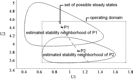
3.2.3 Estimation of the quadratic stability region . . . 44
3.2.4 Discussion . . . 46
3.3 Local stability of the gas turbine with the rotational speed held constant 47 3.4 Summary . . . 48
4 Controller design for a low-power gas turbine 50 4.1 Literature review . . . 50
4.1.1 State space based control methods . . . 50
4.1.2 Control of gas turbines . . . 51
4.2 Control structure selection . . . 52
4.3 LQ servo controller design based on input-output linearization . . . . 54
4.3.1 Control problems and aims . . . 54
4.3.2 Input-output linearization . . . 54
4.3.3 Servo controller with stabilizing feedback . . . 55
4.3.4 Simulation results . . . 57
4.4 MPT controller design based on the LQ controlled plant . . . 60
4.4.1 Control problems and aims . . . 60
4.4.2 Design of the LQ-MPT controller . . . 61
4.4.3 Simulation results . . . 61
4.5 Design of an LQ servo controller with adaptive load torque estimation 63 4.5.1 Control problems and aims . . . 63
4.5.2 Input-output linearization with load torque estimation . . . . 63
4.5.3 Servo controller with stabilizing feedback . . . 66
4.5.4 Simulation results . . . 68
4.5.5 Robustness . . . 68
4.6 Summary . . . 70
5 Determining invariants (first integrals) of QP-ODEs 72 5.1 An algorithm for determining a class of invariants in QP-ODEs . . . 72
5.1.1 The examined class of invariants . . . 72
5.1.2 The underlying principle of the algorithm . . . 73
5.1.3 The basic algorithm for retrieving single invariants . . . 74
5.1.4 Retrieval of multiple first integrals . . . 77 5.1.5 Implementation and computational properties of the algorithms 77
5.2 Algebraic properties of the algorithm . . . 78
5.2.1 The effect of quasi-monomial transformations . . . 78
5.2.2 The effect of algebraic equivalence transformations . . . 79
5.3 Discussion . . . 79
5.4 Examples . . . 80
5.4.1 Example 5.1: A fed-batch fermentation process . . . 80
5.4.2 Example 5.2: A Rikitake system . . . 83
5.4.3 Example 5.3: An electric circuit . . . 84
5.4.4 Example 5.4: A computational example with multiple first in- tegrals . . . 85
5.5 Summary . . . 86
6 Conclusions 87 6.1 Main contributions . . . 87
6.2 Application areas, directions of future research . . . 89
6.3 Publications . . . 90 A Nomenclature, constants and coefficients of the gas turbine model 92 B Zero dynamics of the gas turbine model for the rotational speed 95
C. Tézisek magyar nyelven 97
List of Figures
2.1 General scheme of feedback control . . . 13
3.1 The main parts of a gas turbine . . . 35
3.2 Schematic diagram of the DEUTZ T216 gas turbine . . . 35
3.3 Quadratic stability neighborhood estimation . . . 44
3.4 Transients started from corner points . . . 45
3.5 Quadratic stability neighborhood estimation . . . 46
3.6 Phase diagrams for the system with four different rotational speed values . . . 48
3.7 Phase diagrams for the system with four different load torque values near a typical rotational speed value . . . 48
3.8 Phase diagrams for the system with four different load torque values near minimal and maximal rotational speed values . . . 49
4.1 The input-output linearized plant . . . 56
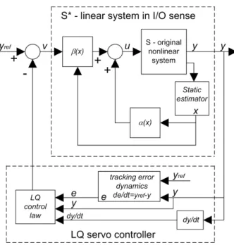
4.2 LQ servo controller on the I/O linearized plant . . . 58
4.3 Reference signal tracking for the rotational speed . . . 58
4.4 Robustness of the LQ servo controller . . . 59
4.5 LQ and MPT controllers on the I/O linearized plant . . . 62
4.6 The effect of step-like changes of load torque on system variables . . . 63
4.7 LQ servo controller on the adaptively I/O linearized plant . . . 67
4.8 Adaptive estimation of the load torque . . . 68
4.9 Robustness of the adaptive LQ servo controller I. . . 69
4.10 Robustness of the adaptive LQ servo controller II. . . 70
5.1 The fed-batch fermenter . . . 80
5.2 The two-disk dynamo system . . . 83
5.3 The LC circuit . . . 84
List of Tables
3.1 State, input, output and disturbance variables of the gas turbine model 41 A.1 Constants of the model of the DEUTZ T216 type gas turbine . . . . 93 A.2 Coefficients of the model of the DEUTZ T216 type gas turbine . . . . 94
Chapter 1 Introduction
If you can’t come across the mountain, walk round it.
If you can’t walk round, fly over it.
If you can’t do this, sit down, and think over whether it is really important to get to the other side.
If so, start to dig a tunnel.
/Maria Fontaine/
1.1 Motivation and background
The analysis and control of nonlinear dynamical systems is an undoubtedly challeng- ing field of systems science. Its significance is well characterized by the number of different practical areas it is applied day by day, for instance in process systems [45], electric power generation [54], robotics [16], transportation systems such as wheeled vehicles [36], aircrafts [77], submarines [78] or spacecrafts [101], and in many other areas of modern life.
A large number of concentrated parameter nonlinear systems can be mathe- matically described by finite dimensional nonlinearinput-affine state space models, where the state equation is a set of ordinary differential equations (ODEs) [46]. This is a definitely advantageous kind of representation, since there are a large number of theoretically well founded tools available for dynamical (stability, controllability, observability) analysis and also for controller design that can be applied thereon (see e.g. [88],[49],[71]). However, the generality of this representation form needs gener- ally applicable (and therefore sometimes less powerful or non-constructive) methods for both dynamic analysis and controller synthesis. Although there are several model classes that have more specialized and practically applicable analysis and synthesis tools that rely on the special model structure, these are usually narrower classes of nonlinear dynamic models and therefore they suffer from the lack of representability.
Fortunately, there is a special physically nonlinear model class in the literature that fit to the nature of certain model classes. The class of quasi-polynomial (QP) models that are also called generalized Lotka-Volterra models has proved to be a unifying nonlinear model class that the majority of the nonlinear models with smooth nonlinearities can be algorithmically transformed to [47]. It is known that QP
system models have several advantageous features that simplify nonlinear dynamical analysis and control techniques: they possess a simple candidate structure for their Lyapunov function [40], [92], moreover their special structure can be exploited in controller design as well [69].
For the modelling, dynamic analysis and control of nonlinear dynamical systems, the special nonlinear nature of the system can be achieved directly: in thermody- namics, mechanics and engineering sciences there is a far amount of nonlinear model information, and one can find ways to exploit this knowledge base. For this purpose a really multi-disciplinary approach is needed that integrates the engineering knowl- edge of the application domain with the appropriate results of nonlinear systems and control theory. Such an approach is traditionally called a grey box methodology [19].
With this grey-box approach, the prior physical insight allows one to model non- linear dynamical systems. A systematic seven step modelling procedure can be found in [46], where the dynamical system is modelled by a mixed set of differential and algebraic equations (DAEs): the differential equations originate from conservation balances for the extensive conserved quantities while the algebraic constitutive equa- tions complete the model. This shows that the general form of the state equations of nonlinear concentrated parameter system models is a system of DAEs. In fortunate cases, the algebraic equations can be eliminated by variable substitution resulting in state equations in ODE form - the differential index of the DAE state equation (i.e. the minimal number of necessary time differentiations to be performed on the algebraic equations to get an ODE state equation) [59] is equal to one in these cases.
However, it occurs quite often that this elimination cannot be performed (strongly nonlinear index-one models or "high index" models, where the differential index is at least two) and the state equation remains in DAE form, and therefore the methods of dynamical analysis and controller synthesis for systems described by state space models in input-affine ODE form cannot be applied. Unfortunately, the dynamical analysis and controller design tools that can be found in the literature generally deal with only very narrow classes, e.g. controller design for DAE mod- els which are only nonlinear in their differential variables [59], or the extension of stability theorems to models where the number of the differential and the algebraic equations are equal [84]. Moreover, the time-differentiation of the algebraic part of these DAEs yield to ODE models that are inherently non-minimal excluding the application of most of the standard dynamical analysis and controller design tools.
While the development of hundreds of years in the theory of differential equa- tions gives a well-founded basis for ’standard’ ODE models, the lack of theoretical background for DAEs makes the analytical treatment of these models difficult. Since a rising number of dynamical models - e. g. models of strongly nonlinear complex systems or high precision models that have an emerging role in a lot of practical fields with an ever-growing demand for punctuality - fall into the class of non-substitutable DAE models, the lack of widely applicable general analysis and controller design methods is a serious and emerging problem that calls for a solution.
1.2 Problem statement and aims
It has been discussed that the QP structure supplies several advantages for both the dynamical analysis and controller synthesis in case of ’classical’ nonlinear ODE state-space models, without the loss of representability. This motivates us to alloy the DAE form with the QP formalism.
This thesis represents the very first steps towards the analysis and control of dynamical systems modelled by nonlinear input-affine DAEs. Three related main topics will be presented that are common in attempting to exploit the advantages of the quasi-polynomial formalism.
The Lyapunov stability analysis of steady state operating points of nonlinear models is not obvious even in the ODE case, since there is no generally applicable constructive method for finding an appropriate Lyapunov function [87]. Lyapunov function candidates can also be used for the estimation of the stability neighborhood (the domain of attraction) of an operating point. There are various methods for doing this for the classical smooth nonlinear ODE state space case [39], however they have limitations in their applicability. The most popular Zubov’s method guarantees the exact knowledge of the domain of attraction, however it needs the solution of a partial differential equation and therefore it is hardly applicable in the general nonlinear case [53]. Based on Zubov’s result, an iteratively computed rational type Lyapunov function is proposed in [97] to estimate the domain of attraction, however its degree (and also the order of the nonlinear model) is limited by the computational complexity of the method. Note that there are well applicable methods developed to narrower system classes, e.g. quadratic Lyapunov functions for polynomial systems [26].
For a special class of rank-deficient QP models, namely Lotka-Volterra mod- els - which are hidden QP-DAEs - there is an algorithmic procedure for finding a quadratic Lyapunov function and estimating the attractor of a steady state point [68]. The first topic aims toapply this method to different zero dynamics of a strongly nonlinear quasi-polynomial model of a low-power gas turbine.
The second topic is directed towards designing controllers of different type for the low power gas turbine. This topic is QP-specific in the sense that the gas turbine model is a QP-DAE with substitutable algebraic equations. Although standard con- troller design methods are to be applied, the special QP structure is to be exploited again.
Finding constants of motion (invariants) of ODE systems is a very complex topic of mathematics, sometimes requiring intimate mathematical skills, usually with a lot of heuristic operations to be performed [3],[82],[90]. Furthermore, it has a great theoretical and practical importance in systems and control theory, because ODE state space models that are not integrable (i.e. have invariant(s)) are generally not reachable (controllable) [49]. The last topic aims to develop a new, algorithmizable method for finding QP type invariants of QP state space models.
1.3 The structure of the thesis
This thesis consists of 6 chapters and an Appendix with two parts. The scientific contributions are contained in Chapters 3,4,5 - each one gives the material of one scientific thesis. The structure of the thesis is organized as follows:
After this introductory chapter, Chapter 2 describes the three main represen- tation types of lumped parameter systems (ODE, DAE and QP state space models) together with their fundamental properties, and introduces the related notions and tools to be used. Key notions, properties and techniques are linked with a literature review.
Chapter 3 concerns with the stability analysis of two zero dynamics of a low power gas turbine model. First, the strongly nonlinear QP-DAE model of the gas turbine taken from literature is presented in Section 3.1. The quadratic stability analysis of the gas turbine with the turbine inlet total pressure held constant is performed in Section 3.2, with the stability region estimation of the operating point.
Section 3.3 concerns with the stability analysis of the gas turbine with the rotational speed held constant.
Chapter 4 is dedicated to controller design for the low power gas turbine.
After a literature review (Section 4.1), control structure selection for the gas tur- bine is performed in Section 4.2 based on the results of Chapter 3. Then, different input-output linearization based controllers are designed: an LQ servo controller in Section 4.3 to track a prescribed reference signal for the rotational speed, and an LQ+MPT controller in Section 4.4 to keep the rotational speed and its time- derivative between predefined bounds. A novel, adaptive input-output linearization based LQ servo controller is designed in Section 4.5 to track a reference signal for the rotational speed, while the most important environmental disturbance of the gas turbine, namely the load torque is estimated dynamically. The performance and robustness of these controllers are tested via simulations performed in the MAT- LAB/SIMULINK computation environment.
Chapter 5 describes a new algorithmic method based on linear algebra that is capable of finding QP type invariants (first integrals) of non-minimal QP-ODE (i.e.
hidden QP-DAE) state space models. Sections 5.1.3 and 5.1.4 describe the retrieval algorithm for single and multiple first integrals, respectively. The computational properties and the implementation of these algorithms in the MATLAB compu- tational environment is discussed in Section 5.1.5. Section 5.2 concerns with the algebraic invariance properties of the algorithms under different transformations.
Finally the operation of the algorithms are demonstrated on several examples in Section 5.4.
Chapter 6 contains the new scientific results in the form of three Theses, the possible directions of future research and the list of own publications.
Appendix A contains the explanation of the variables, coefficients and the values of the nominal parameters of the low power gas turbine model.
Appendix B presents the zero dynamics of the low power gas turbine for the rotational speed.
Appendix C contains the new scientific results in Hungarian.
1.4 Notations
The most important notations and acronyms used throughout the Thesis are enlisted in this section.
Basic mathematical notations
x∈S xis an element of S X ⊂S X is a subset of S
R the set of real numbers
R+ the set of positive real numbers R+0 the set of non-negative real numbers w∈Rn wis a real vector with n components
wi i-th component of vectorw wT transpose of vectorw
f ∈Rn 7→Rm function that assigns vectors of Rm to vectors of Rn
∂f
∂x general Jacobian matrix of functionf ∈Rn7→Rm, x7→f(x)
∂f
∂xi
partial derivative of functionf ∈Rn7→Rm, x7→f(x) byxi
M ∈Rn×m M is a real n×m matrix Mi,j (i, j)-th element of matrix M MT transpose of matrixM
Acronyms
AFLT Adaptive Feedback Linearization Theorem DAE differential algebraic equation
LMI linear matrix inequality LTI linear time invariant
LQ linear quadratic LV Lotka-Volterra
MPT Multi-Parametric Toolbox (used for controller design) ODE ordinary differential equation
QM quasi-monomial
QMT quasi-monomial transformation QP quasi-polynomial
RHS right-hand side
SISO single input - single output
Notations related to state space models
d vector of external disturbances
f state function of nonlinear input-affine system models
g input function of single input nonlinear input-affine system models h output function of input-affine system models
u vector of system inputs x vector of system states y vector of system outputs
A coefficient matrix of QP models, or state matrix of LTI models ALV parameter matrix of LV models
B exponent matrix of QP models, or input matrix of LTI models C exponent matrix of QMTs, or output matrix of LTI models
U vector of state variables of LV models, or vector of QMs of QP models λ parameter vector of QP models
λLV parameter vector of LV models Subscripts
wd refers to dimensionless version of a system variable w wmax refers to maximal value of a system variable w
wmin refers to minimal value of a system variable w wref refers to reference value of a system variable w
w0 refers to initial value of a system variable w Superscripts
¯
w centered version of a system variable w b
w estimated version of a system variable w w∗ steady state value of a system variable w
˙ w= dw
dt time-derivative of a system variable w
Chapter 2
Basic notions and literature review
The purpose of this chapter to get the Reader acquainted with those notions and techniques that should be necessary for the understanding of the following chapters.
These notions and tools are collected around the three main system model forms (ODE, DAE and QP) that will be used in this Thesis.
2.1 State equations in the form of ordinary differ- ential equations (ODEs)
The majority of nonlinear lumped parameter systems with smooth nonlinearities can be represented in the form of ordinary differential equations (ODEs). As we will see, this purely differential form has the great advantage that dynamic analysis and plenty of controller design techniques are developed for it [45]. This section concerns with the dynamical (stability and reachability) analysis and shows several controller design techniques for systems represented in ODE form.
2.1.1 Linear time invariant (LTI) system models
First, let us get acquainted with the LTI state space representation consisting of an ODE state equation and a linear output equation:
˙
x = Ax+Bu (2.1)
y = Cx+Dy (2.2)
where x∈Rn, u∈Rp, y ∈Rq are the vectors of state, input and output variables, respectively, A ∈ Rn×n, B ∈Rn×p, C ∈ Rq×n are constant matrices. It is important to note that an n-th order state space model is never unique: there are infinitely many n-th order state space models describing the same system [44].
The importance of LTI system models is twofold: a lot of nonlinear ODEs can be transformed to an LTI one with an appropriate control input function, giving rise to the application of linear controllers on the linearized model, moreover LTI models are often derived from nonlinear state space models by local linearization around a steady state operating point.
2.1.2 Nonlinear input-affine system models
As an advantageous mathematical representation for lumped parameter systems, the nonlinear input-affine state space model is proposed [45].
Nonlinear state space models are described by vector fields which are construc- tions in vector calculus [29]. A vector field associates a vector to every point of an Euclidean space. Thus, a vector fieldH that associates ad2 dimensional real vector to each point of the d1 dimensional real coordinate space can be represented as a vector valued function:H :Rd1 →Rd2.
A vector field H is calledaffine inw= [w1, . . . , wk]T if its vector valued function representation H(v, w) can be written in the form
H(v, w) = F(v) + Xk
j=1
Gj(v)wj
whereF andGj, j = 1, . . . , k are arbitrary vector valued functions. The term input- affine system model denotes a system model that is affine in the input variables.
Let us denote the vector of states by x ∈ χ, where χ is an open subset of Rn, the vector of system inputs byu∈Rp and the vector of system outputs by y∈Rq. The general input-affine form consists of a state equation in the form of an ordinary differential equation (ODE), and an output equation [45]:
˙
x = dx
dt =f(x) + Xp
i=1
gi(x)ui (2.3)
y = h(x) (2.4)
where f, gi ∈Rn7→Rn, i= 1, . . . , p and h∈Rn 7→Rq are smooth nonlinear vector fields (i.e. their vector valued function representations are smooth and nonlinear), and u= [u1, . . . , up]T.
2.1.3 Asymptotic stability of nonlinear input-affine systems
This section deals with the notion and investigation methods of asymptotic stabil- ity. Together with the local (eigenvalue checking) method, the main objective is to discuss how to investigate the asymptotic stability of nonlinear systems by means of the widely used Lyapunov-technique [49].
Determine the input u of the nonlinear input affine state equation (2.3) as a function of x (i.e. apply a control law that is in the form of u = ψ(x)) or simply truncate it by setting the input to zero (u= 0). Then (2.3) becomes an autonomous ODE that can be written in a ’controlled’ (’closed loop’) or ’truncated’ form
˙ x= dx
dt =fa(x) (2.5)
where fa ∈Rn7→Rn is again a smooth nonlinear vector field.
Consider the autonomous nonlinear ODE in (2.5). We call x∗ an equilibrium point (or steady state point) of (2.5) if it fulfills the equation
fa(x∗) = 0
e.g. dtdx∗ = 0. Denote x0 =x(0) the initial condition of (2.5).
- An equilibrium point x∗ of (2.5) is called stable in Lyapunov sense, if for arbitraryǫ >0there is aδ >0such that if||x0−x∗||< δ then||x(t)−x∗||< ε for every t >0, where|| · || is a suitable vector norm.
- An equilibrium point x∗ is called asymptotically stable, if it is stable in Lya- punov sense, andlimt→∞x(t) = x∗.
- If x∗ is not stable, it is called unstable.
- We call x∗ locally (asymptotically) stable, if there is a neighborhood U 6=Rn of x∗, wherex∗ is (asymptotically) stable.
- If x∗ is (asymptotically) stable in Rn, then x∗ is a globally (asymptotically) stable equilibrium of (2.5).
As we can see, stability (asymptotic stability) is a property of equilibrium points in case of nonlinear ODEs. However, the stability (asymptotic stability) of the n- th order LTI system model (2.1)-(2.2) is a system property, since it is realization independent: any other n-th order state space models describing the same system as (2.1)-(2.2) are stable (asymptotically stable). Moreover, stability (asymptotic stability) is always global in the LTI case. Note that if (2.1)-(2.2) is asymptotically stable, then its equilibrium point is unique: it is the origin of the state space, i.e.
x∗ = 0∈Rn.
The asymptotic stability of LTI system models can easily be checked by the eigenvalues of its state matrix A: (2.1)-(2.2) is asymptotically stable if and only if Re(λi(A)) < 0, i = 1, . . . , n, where the eigenvalues λi, i = 1, . . . , n of A are the solutions of the equation
det(λI−A) = 0
where I ∈ Rn×n is the unit matrix [44]. In addition, if Re(λi(A)) > 0 for some i, then (2.1)-(2.2) is unstable. It is important to note that if Re(λi(A)≤0 and there is at least one eigenvalue with zero real part, then stability can be checked in the following way: Let (2.1)-(2.2) have s different eigenvalues with zero real parts. If the eigenvectors belonging to theses eigenvalues span an s-dimensional space, then (2.1)-(2.2) is stable (not asymptotically!), otherwise it is unstable. Note that the (non-asymptotic) stability of LTI system models is also a system property.
This eigenvalue-checking method can be extended to nonlinear input affine sys- tem models: ifx∗ is an equilibrium of (2.5) and the locally linearized model of (2.5) around x∗ is asymptotically stable (unstable), then x∗ is a locally asymptotically stable (unstable) equilibrium of (2.5). Although this method is easily applicable, it does not give us any information about the asymptotic stability neighborhood of the equilibrium point, moreover it can prove asymptotic stability and instability, but it does not give us any information if the locally linearized model has eigenvalue(s) with zero real part(s).
Lyapunov theorem
The most widely used technique for the (global) stability analysis of nonlinear input- affine systems is the so-called Lyapunov technique. For proving asymptotic stability of the nonlinear system (2.5) Lyapunov functions are used. These functions can be regarded as "generalized energy" functions, since they are scalar valued, positive definite functions. If the system (2.5) is asymptotically stable, then this energy decreases with time. Therefore a Lyapunov functionV(x)has to fulfill the following criteria:
1. V is a scalar function of the state variables of (2.5):
V ∈ Rn→R+
0
2. V(x)is positive definite at the equilibrium x∗:
V(x)>0 if x6=x∗, V(x∗) = 0 3. Its time-derivative is negative definite at the equilibrium x∗ :
dV
dt = ∂V
∂x dx
dt <0 if x6=x∗, dV
dt = 0, if x=x∗
The Lyapunov-theorem states that the system (2.5) is asymptotically stable if there exists a Lyapunov function with the properties above.
Note that finding an appropriate Lyapunov function is not constructive in gen- eral. However, there are system classes where Lyapunov functions can be given constructively, e.g. in LTI case [44], or for linear parameter varying systems (see e.g.
a control relevant application in [86], or for Hamiltonian systems [43]).
2.1.4 Reachability and minimality of input-affine systems
In this section another dynamical property, namely the reachability will be discussed.
An LTI state space model in the form of (2.1)-(2.2) is called reachable, if it is possible to drive an arbitrary statex(t1)∈χto an arbitrary state x(t2)∈χwith an appropriate input function, in finite time t = t2 −t1. Reachability is always global in the LTI case.
The input-affine state space model (2.3)-(2.4) is said to be locally reachable around the state x(t1)∈χ, if there exists a neighborhood U ⊂χ of x(t1) such that it is possible to drive x(t1) to an arbitrary state x(t2) ∈ U with an appropriate control input function, in finite time t=t2−t1.
The reachability of state space models is a necessary condition for the application of most of the controller design techniques.
An LTI system model in the form of (2.1)-(2.2) is reachable if and only if its controllability matrixC = [BAB . . . An−1B]is of full rank. Note that reachability of LTI system models is also termed as controllability, but to avoid any trouble about notions the term ’reachability’ will be used uniformly throughout this Thesis.
The reachability of the nonlinear input-affine system model (2.3)-(2.4) can also be investigated by an algorithm [49].
Before presenting this algorithm we have to get acquainted with some notions.
Letf, g∈Rn →Rnbe two smooth vector fields. Denote the general Jacobian matrix of f by ∂f∂x:
∂f
∂x =
∂f1
∂x1
∂f1
∂x2 . . . ∂x∂f1
∂f2 n
∂x1
∂f2
∂x2 . . . ∂x∂f2 ... ... ... ...n
∂fn
∂x1
∂fn
∂x2 . . . ∂f∂xnn
, where f =
f1
f2
...
fn
A Lie-bracket (or Lie product) of f and g is another vector field [f, g] ∈Rn → Rn defined as
[f, g](x) = ∂g
∂xf(x)− ∂f
∂xg(x)
A distribution is a function that assigns a subspace of Rn for each point x∈U, where U is an open subset of Rn. A distribution ∆ can be regarded as a subspace depending on x, that is spanned by some vector fieldsδ1, . . . , δd at each point x:
∆(x) = span{δ1(x), . . . , δd(x)}
The algorithm proposed by [49] computes the so-called reachability distribution, using Lie-brackets.
• The initial step is:
∆0 =span{gi, i= 1, . . . , q}
• The k-th step of the algorithm is the following. Let ∆k−1 = span{δj(k−1), j = 1, . . . , d}. Then∆k is computed as
∆k =span{δj(k−1),[f, δ(k−1)j ],[gi, δj(k−1)] , i= 1, . . . , p, j = 1, . . . , d} (2.6)
• The stopping condition of the algorithm is: dim(∆k∗) =dim(∆k∗−1) for some k∗.
The distribution∆ = ∆k∗ is called the reachability distribution of (2.3)-(2.4). Since the maximal dimension of ∆is n, the algorithm consists of finite steps.
If the dimension of the reachability distribution is maximal at a point x0 ∈ χ, i.e. dim(∆(x0)) = n, then there is a neighborhood U0 of x0 such that (2.3)-(2.4) is reachable locally on U0. If dim(∆) = n independently of x, then (2.3)-(2.4) is (globally) reachable.
A state space model is called minimal, if its dynamics is described by the mini- mum number of state variables (i.e. the dimension of the state space (n) is minimal) [49]. It is known that a state space model is minimal if and only if it is reachable and observable. Observability roughly means that the exact knowledge of the input and output signals and also of the state space model is enough to determine the state trajectories of the system.
Thus, the non-minimality of (2.3)-(2.4) might mean that there are hidden alge- braic constraints on the state variables, which is the subject of the next section.
2.1.5 Invariants (first integrals) of ODE models
A function I : Rn 7→ R is called an invariant (constant of motion, first integral or hidden algebraic constraint) of the non-autonomous ODE defined in (2.3) if
d
dtI = ∂I
∂x ·x˙ = 0. (2.7)
The determination of invariants of ODEs has been occupying scientists’ mind for the last 100 years. As the most frequent and widely used approaches, methods based on Lie-symmetries [90] and Painlevé analysis [3],[82] has to be mentioned.
Unfortunately, these methods are not applicable for arbitrary types of first integrals - see e.g. [76] that concerns with invariants that cannot be determined using Lie- symmetries. Additionally, their often heuristic and generally symbolic nature makes the determination of the invariants difficult.
First integrals play a great role in modern systems and control theory e.g. in the field of canonical representations, reachability and observability analysis [49]
and also in the stabilization of nonlinear systems [88],[63]. Moreover, if the given dynamical system is not integrable, then its first integrals (if they exist) give us very useful information about the properties of the solutions and about physically meaningful conserved quantities.
If an ODE state space model has first integral(s), then it is indeed non-minimal because its dynamics can be described with a lower number of state variables. More- over, its state trajectories evolve on a manifold (i.e. a lower dimensional subset of the state space) determined by its first integral(s). As a consequence, these state space models are not reachable, since only the states on the manifold determined by the invariant(s) can be reached. It has to be emphasized that from the fact that (2.3) with zero inputs (ui = 0, i = 1, . . . , p) has an invariant does not imply that (2.3) with arbitrary inputs also has this invariant, since e.g. a state feedback may result a completely different autonomous ODE. However, there are invariants that cannot be influenced by the control input.
For systems in the form (2.3-2.4) Isidori proposes a method to determine first integrals [49] that are independent of the control input variable. The complexity of this method is well characterized by the fact that it demands the symbolic solu- tion of systems of partial differential equations (PDEs). These difficulties are well demonstrated on the reachability analysis of a low (third) order fermentation pro- cess model needing the solution of a system of two PDEs. There are other methods that consider model classes that can only represent a narrower class of lumped pa- rameter systems: e.g. positive systems [63], polynomial systems [67], or single n-th order nonlinear ODEs [4].
2.1.6 Control of nonlinear input-affine systems
This section is dedicated to introduce control techniques and control relevant notions that will be used throughout the Thesis.
Theaim of control is tomodify a system in such a way that it fulfills aprescribed control goal. This modification is usually done by a feedback: the input variable uof the system is determined as a function of the signals (the outputs and/or the states)
of the system (see Fig. 2.1). A system with a feedback controller is often called as closed loop system, in contrast to the uncontrolled, open loop system.
Feedback controllers can be classified by their properties. A feedback can be - a state/output feedback, if it uses the state/output signals of the system;
- linear/nonlinear if it is a linear/nonlinear function of the signals (outputs, states) of the system;
- dynamic, if it also contains the derivatives of the states/outputs of the system, and static otherwise;
- a full state feedback, if all components of the state variable vector are used in the computation of the state feedback.
SYSTEM
CONTROLLER states x
inputs u outputs y
y x u=F(x,y)
Figure 2.1: General scheme of feedback control
In the following, a few different types of feedback controllers will be described.
Linear quadratic (LQ) and LQ servo controllers
LQ and LQ servo controllers can be applied to LTI models in the form of (2.1)-(2.2), but they can also be applied to (locally or globally) linearized nonlinear input-affine models. (The input-output linearization of nonlinear input affine models will be discussed in the next section.) LQ and LQ servo controllers use linear static feedback.
In the following, we focus on LQ controllers with full state feedback.
The problem statement of LQ control is the following: Given an LTI state space model in the form (2.1)-(2.2). Minimize the following functional (the control cost)
J(x, u) = 1 2
Z T
0
xT(t)Qx(t) +uT(t)Ru(t)dt (2.8) by an appropriate input u(t), t ∈ [0, T], where Q and R are positive definite, sym- metric weighting matrices for the states and inputs, respectively.
If (2.1)-(2.2) is reachable and observable (i.e. from the exact knowledge of system parameters,u(t)andy(t), the statesx(t)can be determined), the stationary solution
(i.e. whenT → ∞) of this control problem can be obtained by solving the so-called Control Algebraic Ricatti Equation for P:
ATP +P A−P BR−1BTP +Q= 0 (2.9) It is known that this matrix equation has a unique positive definite symmetric solutionK [44]. Then, the static linear full state feedback
u(t) =−Kx(t) =−R−1BTP x(t) (2.10) minimizes the functional (2.8) if T → ∞. The weighting matrices Q and R are the tuning parameters of the LQ controller. The quadratic termxTQxin (2.8) penalizes the deviation of the state vector from the reference state x∗ = 0, while the other quadratic term uTRu penalizes the control energy. The magnitude of elements in Q and R can be chosen according to the control aim: choosing a Q that is relatively
’big’ compared toR, the deviations from the zero state are smaller, however it needs more input energy (cheap control), while with aQthat is relatively ’small’ compared toR the transients of the controlled plant have higher deviations while the control need less energy (expensive control). It is important to note that an LQ controller designed to an arbitrary LTI model guarantees the asymptotic stability of the closed loop system independently of the design parametersQandR. Another advantage of LQ controllers is that the closed loop system is robust against some model parameter uncertainties and environmental disturbances [45].
While LQ controllers make the system track the prescribed trajectory x(t) = 0, LQ servo controllers are designed to track a prescribed reference output signal yref(t). Consider the simplest case, when (2.1)-(2.2) is a cascade of integrators:
˙
x1 = x2
˙
x2 = x3
...
˙
xn−1 = xn
˙
xn = u y = x1
This can be re-written in matrix-vector form:
dx dt =
0 1 0 . . . 0 0 0 1 . . . 0 ... ... ... ... ...
0 0 0 . . . 1 0 0 0 . . . 0
x(t) +
0 0...
0 1
u(t) (2.11)
y(t) =
1 0 0 . . . 0
x(t) (2.12)
Compute an LQ state feedback in the form
u(t) =−Kx(t) = −k1x1(t)−k2x2(t)−. . .−knxn(t)
The closed loop system can be written in the form
dx dt =
0 1 0 . . . 0
0 0 1 . . . 0
... ... ... ... ...
0 0 0 . . . 1
−k1 −k2 −k3 . . . −kn
x(t) (2.13)
y(t) =
1 0 0 . . . 0
x(t) (2.14)
Recall that since this closed loop system is asymptotically stable, it asymptotically tracks the reference statex∗ = 0.
This closed loop system has to be modified in such a way that y = x1 has to track the prescribed reference signal yref(t), therefore the state to be tracked is x∗ref(t) = [yref(t) 0 . . . 0]T. Define the tracking error as
e(t) =yref(t)−y(t) =yref(t)−x1(t) Modify the LQ control law as
u(t) = −k1(−e(t))−k2x2(t)−. . .−knxn(t) =
= −k1(x1(t)−yref(t))−k2x2(t)−. . .−knxn(t) =−Kx(t) +k1yref(t)(2.15) This control law applied to (2.11) guarantees thatlimt→∞e(t) = 0 if limt→∞yref(t) exists; and therefore x1(t) asymptotically tracks yref(t).
The LQ servo controlled cascade of integrators can be written in the following matrix-vector form:
dx dt =
0 1 0 . . . 0
0 0 1 . . . 0
... ... ... ... ...
0 0 0 . . . 1
−k1 −k2 −k3 . . . −kn
x(t) +
0 0...
0 k1
yref(t) (2.16)
y(t) =
1 0 0 . . . 0
x(t) (2.17)
If (2.1)-(2.2) is not a cascade of integrators, an LQ servo controller can be built by defining the tracking error e by a new differential equation:
˙
e=yref(t)−y(t) =yref(t)−Cx(t) (2.18) This yields to the following (n+ 1) dimensional LTI model:
d dt
e(t) x(t)
=
0 −C 0n×1 A
e(t) x(t)
+
0 B
u(t) + 1
0n×1
yref(t) (2.19)
y(t) = Cx(t) (2.20)
where0is a single zero element,0n×1 is anndimensional zero vector, whileA,Band C are the matrices of the LTI model (2.1)-(2.2). An LQ feedback applied thereon in the form
u=−kee(t)−k1x1(t)−. . .−knxn(t)
guarantees the asymptotic stability of the system, moreover - if y(t) =x1(t) - then x1(t) asymptotically tracks yref(t).
Note that the advantageous properties of LQ controllers (stability, robustness) stand for LQ servo controllers, too.
Constrained linear optimal control
LQ controllers do not guarantee that the different signals: the states, outputs, and the control input computed by the controller are bounded, however it is a significant criteria in many physical systems.
The constrained linear control technique (see, e.g. [17], [18], [20]) solves this problem for LTI systems. Constrained linear optimal control considers the following discrete time SISO LTI system class:
x(k+ 1) = Ax(k) +Bu(k)
y(k) = Cx(k) +Du(k) (2.21)
where k = 0,1, . . . is the discrete time, x(k)∈Rn is the state vector, u(k)∈R and y(k)∈R are the input and output respectively.A, B, C and D are real matrices of appropriate dimensions. Note that a discrete time LTI model in the form (2.21) can be obtained from a continuous LTI model (2.1)-(2.2) by time-discretization [44].
The so-called Constrained Finite Time Optimal Control Problem with quadratic cost is to find an input sequence {u(0), . . . , u(N −1)} such that it minimizes the cost function
J(x, u) = x(N)TPNx(N) +
N−1X
k=1
[u(k)TRcu(k) +x(k)TQcx(k)] (2.22) subject to the constraints
umin ≤u(k)≤umax (2.23)
ymin ≤y(k)≤ymax (2.24)
Hx(k)≤K (2.25)
where PN, Qc and Rc are positive definite symmetric weighting matrices (design parameters), H ∈ Rl×n and K ∈ Rl are matrices defining a prescribed polytopic region of the state space inside which the state variables have to evolve.
The constrained linear optimal control problem can be solved by multi- parametric programming. For the numerical solution, the Multi-Parametric Toolbox (MPT) [61] of the MATLAB computational environment has been used.
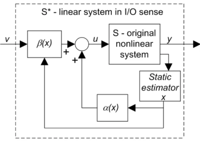
Input-output linearization of nonlinear input-affine systems [49]
Input-output linearization is the application of an appropriate nonlinear state feed- back to obtain a system description which is linear in input-output sense. Consider the general nonlinear input-affine system model in (2.3)-(2.4) with single input and
single output:
˙
x = dx
dt =f(x) + Xp
i=1
g(x)u (2.26)
y = h(x) (2.27)
where x ∈ χ ⊂ Rn, u, y ∈ R and f, g ∈ Rn 7→ Rn and h ∈ Rn 7→ R are smooth nonlinear vector fields.
The relative degree of (2.26)-(2.27) at a point x0 ∈χis a nonnegative integer r, that fulfills the following conditions:
1. LgLkfh(x) = 0 for all x in a neighborhood of x0 and k < r−1 2. LgLr−1f h(x)6= 0
where Lfh(x), Lkfh(x) denote Lie derivatives Lfh(x) =L1fh(x) = ∂h
∂xf(x) , Lkfh(x) = LfLk−1f h(x) , k= 2,3, . . .
In other words, the relative degreeris the minimum number of time differentiations that has to be performed on the output y to get the inputu explicitly appear.
The zero constrained output dynamics - or zero dynamics in brief - of (2.26)- (2.27) is the dynamics of (2.26) that fulfills the constraint
y(t)≡0
If the relative degree of (2.26)-(2.27) is r in a neighborhood of x0, then its zero dynamics is n−r dimensional. If n=r, then the system has no zero dynamics.
Let the relative degree of the system (2.26)-(2.27) be r < n at a neighborhood of x0 ∈ χ. Apply the following nonlinear coordinates transformation in the neigh- borhood of x0:
z =T(x) =
h(x) Lfh(x)
...
Lr−1f h(x) ϕ1(x)
...
ϕn−r(x)
(2.28)
where ϕi(x), i = 1, . . . , n−r are chosen in such a way that they fulfill Lgϕi(x) = 0, i= 1, . . . , n−r aroundx0.
By applying the following input function u=α(x) +β(x)v, α=− Lr−1f h(x)
LgLr−1f h(x), β = 1
LgLr−1f h(x), (2.29)
the nonlinear input affine system model in (2.26)-(2.27) can be rewritten in the new coordinates [49]:
˙
z1 = z2
˙
z2 = z3
...
˙
zr = v
˙
zr+1 = Φ1(z) ...
˙
zn = Φn−r(z) y = z1
where v is the new input variable. The transformed system is split into a linear r-dimensional subsystem (a cascade of integrators), and a nonlinear (n−r) dimen- sional subsystem. Observe that the nonlinear subsystem - which is exactly the zero dynamics - is independent of the new input v and does not appear in y, therefore the system in the transformed coordinates is linear in input-output sense.
Since this zero dynamics does not depend on the control input, only the linear subsystem can be and should be controlled. This gives rise to the application of linear controllers. The great advantage of this input-output linearized form is that if the zero dynamics is asymptotically stable, then with arbitrary asymptotically stabilizing feedback (e.g. an LQ controller) the whole system becomes asymptotically stable [49].
Also note that if the relative degree of the system is n near x0 ∈ χ, the system (2.26)-(2.27) has no zero dynamics and is calledfeedback linearizable near x0: it can be re-written in the new coordinates as a cascade of integrators.
Adaptive feedback linearization [71]
The adaptive feedback linearization method performs feedback linearization and handles model parameter uncertainties at the same time.
Consider a variant of the input affine single input-single output (SISO) nonlinear input affine state space model in (2.26)-(2.27):
˙
x = dx
dt =f(x) + Xs
i=1
qi(x)µi+g(x)u (2.30)
y = h(x) (2.31)
whereµ= [µ1, . . . , µs]T ∈Rs is the vector of unknown constant parameters. Denote the adaptive estimation of the unknown parameter vectorµ byµˆ∈Rs.
Theproblem statement of the adaptive feedback linearization [71] is the following:
Given a reference model
˙
zr =Arzr+Brvr , zr ∈Rn, Ar =
0 1 0 . . . 0
0 0 1 . . . 0
... ... ... ... ...
0 0 0 . . . 1
−k1 −k2 −k3 . . . −kn
(2.32)
where Br ∈ Rn×1, Ar ∈ Rn×n, (2.32) is asymptotically stable and reachable. Find an adaptive feedback linearizing control for (2.30)-(2.31) which is a dynamic state feedback
d
dtµˆ = ϑ(x, zr, vr,µ)ˆ , µˆ ∈Rs,µ(0) = ˆˆ µ0 (2.33)
u = u(x, zr, vr,µ)ˆ (2.34)
that for any initial conditions x(0),µ(0), zˆ r(0), any unknown parameter µ and any boundedvr(t) fulfills the following requirements:
1. ||x(t)||and||µ(t)ˆ ||are bounded for t≥0, where|| · || is a suitable vector norm;
2. there exist a filtered transformation (i.e. a time-varying coordinates transfor- mation) in the formx=T(z, zr(t),µ(t))ˆ such that
limt→∞||x(t)−T(z, zr(t),µ(t))ˆ ||= 0
Denote ∆k the distribution in (2.6) (this is the result of the k-th step of the algorithm for computing the reachability distribution of input-affine systems). The Adaptive Feedback Linearization Theorem [71] states that if
1. the nominal system of (2.30)-(2.31) (i.e. the system with µ = 0) is globally feedback linearizable,
2. the global triangularity conditions [µi, δj(k)] ⊂ ∆k, are satisfied, where i = 1, . . . , s, k = 0, . . . , n−2, and ∆k =span{δ(k)j , j = 1, . . . , d},
then there exists an adaptive feedback linearizing control.
The construction of this adaptive feedback law is not presented here, since it depends on the ordernof the system, but will be described in detail on the adaptive controller synthesis applied to the low-power gas turbine in Section 4.5.
However, the assumption that µ is constant can be relaxed, if its time behavior can be modelled by an exosystem with unknown initial condition µ(0) [71]:
d
dtµ= Ω(t, x)µ+ω(t, x) (2.35) with the property that
1. Ω(t, x) + ΩT(t, x) is negative semidefinite, t≥0,∀x∈Rn,
2. the exosystem (2.35) has bounded state trajectories µ(t), t≥0 if x(t), t ≥0 is from a bounded set of Rn.
Linear matrix inequalities
Linear matrix inequalities play an important role in the control (an also in the analysis) of dynamical systems. A (non-strict) linear matrix inequality (LMI) is an inequality of the form [89]:
F(x) =F0+ Xm
i=1
xiFi ≥0, (2.36)
where x ∈ Rm is the variable and Fi ∈ Rn×n, i = 0, . . . , m are given symmetric matrices. The inequality symbol in (2.36) stands for the positive semi-definiteness of F(x). LMIs form a convex constraint on the variables i.e. the set
{x | F(x)≥0} (2.37)
is convex. A wide variety of different problems (linear and convex quadratic inequal- ities, matrix norm inequalities, convex constraints etc.) can be written as LMIs and there are computationally stable and effective (polynomial time) algorithms for their solution [21], [89].
2.2 State equations in the form of differential alge- braic equations (DAEs)
This section concerns with DAE models which are the general representation forms of lumped parameter systems. The stability and reachability of these DAE models are also discussed. A short literature review on the control techniques applied for DAEs can also be found at the end of this section.
Lumped parameter systems are usually modelled by a mixed set of (ordinary) differential and algebraic equations (DAEs). The differential equations describe the dynamics of conserved quantities, while the algebraic equations define static rela- tionships and complete the model.
For example, lumped parameter process systems are intuitively modelled by DAEs, following a systematic modelling procedure based on first engineering prin- ciples [46]. The differential equations are balance equations of masses and energies, while the algebraic equations are thermodynamic laws, empirical correlations etc.
Modelling with DAE system models is generally used e.g. for electric circuits, interconnected systems, constrained dynamics etc. DAE system models are also called as singular, semi-state, descriptor or generalized systems, and the notion of singularly perturbed system is also related with DAEs [59].
An equivalent ODE model can be obtained from a DAE model, if - with a sym- bolic Gauss elimination - the algebraic variables can be expressed from the algebraic equations as functions of the differential variables, since then these equations can be eliminated by substituting them to the differential equations. However, for some DAE models the elimination of the algebraic equations is not possible because of the structure of the algebraic equations (e.g. strong nonlinearities, high number of variables). This gives rise to the (possibly iterative) time-differentiation of the alge- braic equations, in order to get a purely differential (ODE) model. Unfortunately,
because of the increased number of differential variables the resulted ODE will be non-minimal, making the dynamical analysis much more difficult, moreover exclud- ing the possibility of the application of standard nonlinear controller design methods.
This problem brings up the need to somehow extend the nonlinear dynamic analysis and control methods to DAE system models.
2.2.1 The general DAE representation of lumped parameter system models
As the first attempt, LTI DAEs have been invented in the literature called as "gen- eralized linear systems" or "descriptor systems" (see e.g. [98]):
Ex˙ = Ax+Bu , x(0) =x0 (2.38)
y = Cx (2.39)
where x, u, y denote the state, input and output vectors of dimensions n,p and q, respectively, while E, A, B, C are matrices of appropriate dimensions and E is a singular (non-invertible) matrix (without this condition the model above becomes an LTI ODE model in the form (2.1)-(2.2) by pre-multiplying both sides of (2.38) by E−1). With a decomposition, which is a linear transformation on the state variable vector x, (2.38)-(2.39) can be split to a set of n1 differential equations and a set of n2 algebraic equations, where n1 +n2 = n [59]. The transformed state variable vector is also split to n1 differential and n2 algebraic variables.
However, for the representation of lumped parameter systems the general repre- sentation form has to cope with nonlinearities, and also with cases when the algebraic variables cannot be expressed explicitly from the algebraic equations. The following, so-called semi-explicit DAE can fulfill these requirements and therefore it can be regarded as the general representation form of lumped parameter systems:
˙
x = f(x, z) + Xp
i=1
gi(x, z)ui (2.40)
0 = w(x, z) (2.41)
y = h(x, z) (2.42)
where x ∈ Rn1 and z ∈ Rn2 are the vectors of the differential and the algebraic variables, respectively, f, gi ∈ Rn1+n2 7→ Rn1, i = 1, . . . , p, w ∈ Rn1+n2 7→ Rn2 and h∈Rn1+n2 7→Rqare smooth nonlinear vector fields, andu= [u1, . . . , up]T is the vec- tor of control input variables. Thestate variables of this DAE consists ofthe vector of differential and the vector algebraic variables. This model is nonlinear and input- affine. The algebraic equations are in implicit form and do not contain control input variables. Moreover, we assume that the initial conditions of the model(x(t0), z(t0)) fulfill the algebraic equations to avoid impulsive solutions. (This assumption could not be done in case of non-smooth functions f, w and gi, i = 1, . . . , p, e.g. in mod- elling electric circuits with switches [98].)