Adaptive Control of Smooth Nonlinear Systems Based on Lucid Geometric
Interpretation
By
József K. Tar
Óbuda University
John von Neumann Faculty of Informatics Institute of Intelligent Engineering Systems
Submitted for the degree of
“Doctor of the Hungarian Academy of Sciences”
Category:
“Technical Science”
2010
Acknowledgments
I should like to to express my thanks to my very much esteemed teachers who gave me impetus in various stages of my studies to develop interests in science.
I have to express my especial thank to professor János Bitó who is my mentor since the middle of the eighties of the past century in the industrial relationships (at TUNGSRAM Co. Ltd.) as well as in the academic sphere even in these days, too. I must be especially grateful to professor Imre Rudas who was my professional leader and in many cases active co-worker in various national and international R&D projects. On similar reason I have to express my personal thanks to professor José António Tenreiro Machado of Institute of Engineering, Porto, Portugal, and professor Krzysztof Kozłowksi of Poznan University of Technology, Poznan, Poland.
Finally I should like to thank the patience, kindness, and continuous support of my already deceased parents who always let me do what I believed to be aesthetic and important in my life.
Abstract
The objective of this dissertation is to give a summary of a research work aiming at the use of simple, geometrically well interpretable mathematical means in the adaptive control of partially and imperfectly modeled nonlinear systems. Such systems may have dynamic coupling with hidden subsystems and may also be under a priori unknown external disturbances.
The novelty in this research consists in the fact that it did not want to proceed in the well established ruts of using Lyapunov functions. Lyapunov’s 2nd or “direct”
method seems to dominate contemporary nonlinear control worldwide. Though the fundamentals of this technique have lucid geometric interpretation, finding a proper Lyapunov function candidate for a given problem is a kind of “art”. Furthermore, guaranteeing its non-positive time-derivative needs intricate mathematical manipulations that need great technical skills. Normally, these parts of the proofs take whole pages in the papers, and they usually result in special conditions that have to be met for the stability of the controllers. As it will be emphasized in this dissertation, the so obtained controllers may contain too much more or less arbitrary parameters. Furthermore, they do not result in optimal tuning. Certain adaptive solutions that try to exactly learn the analytical model of the system under control are vulnerable by the effects of unknown external disturbances and hidden, coupled subsystems.
To avoid the difficulties related to the application of Lyapunov’s 2nd method I tried to utilize very simple and lucid geometric structures and convergent iterations obtained from contractive maps to construct adaptive controllers.
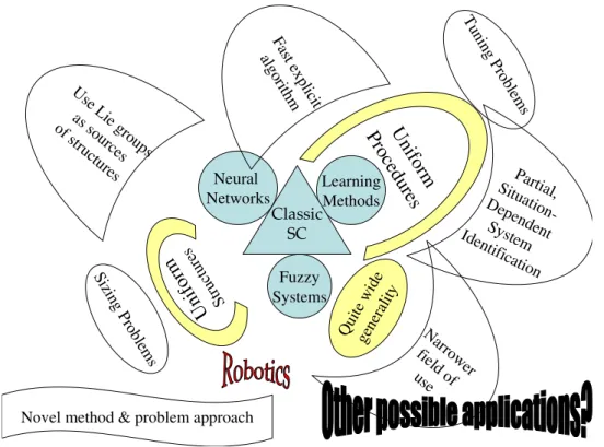
The basic philosophy of this approach is similar to that of the prevailing soft computing techniques. However, it does not apply the typical uniform structures of the modern soft computing that are related to Kolmogorov’s approximation theorem proved in 1957. Instead approximating continuous functions my approach approximates a far better behaving set of smooth functions by utilizing uniform structures of small sizes taken from various Lie groups.
After giving a brief historical review on the advantages of “geometric way of thinking” the Computed Torque Control in Robotics and Lyapunov’s 2nd Method in general and its illustrative applications in Robotics are critically studied and modified. Following that the subject area of soft computing as a special application of universal approximators is critically studied. The emphasis is on the sizing and scalability problems that generate difficulties in parameter tuning.
Instead using “universal approximators” various special elements of special Lie groups are suggested to the realization of partial, temporal, and situation- dependent system identification. The first approach is based on the phenomenological basis of Classical Mechanics in the control of Classical Mechanical Systems. The second one uses these structures at higher level of abstraction. It is shown that these structures have limited number of tuneable parameters and they can be used for the approximation of the observed behavior of the system under control.
In the next research phase various parametric Fixed Point Transformations were proposed for adaptive control to further release the problem of the complexity of system-identification. The geometric interpretation of the Singular Value Decomposition (SVD) of real matrices is also utilized in these approaches. In contrast to Lyapunov’s 2nd method that normally guarantees global stability of the control, in the new approach the convergence of the iteration that is necessary for
cases the basin of convergence is wide enough for practical applicability of the proposed novel methods. Furthermore, it is shown that the novel approach using
“Robust Fixed Point Transformations” can be completed by various parameter tuning methods that are able to keep the controller nearby the center of the basin of attraction of the necessary iteration. This approach works only with three adaptive control parameters of which only one parameter has to be tuned. It also is shown that this tuning is not drastically coupled with the dynamics of the tuning-free controller. It slightly affects the speed of convergence of the iteration and the tracking precision of the tuned adaptive controller.
It also is shown that by the use of this novel adaptive approach a new branch of the “Model Reference Adaptive Controllers” can be developed in the design of which the Lyapunov function can be replaced by the simple Robust Fixed Point Transformations.
Finally, a simple parametric numerical approximation of Caputo’s fractional order derivatives is presented and applied in nonlinear control for smoothing purposes.
The dissertation contains an “Appendix” that summarizing the most important geometric and group theoretical analogies that are utilized in the Thesis. To maintain the page limitation formally prescribed for the “core” material certain mathematical details and numerical computational results are presented in the Appendix, too.
The dissertation separately contains the author’s own publications strongly related to the results given in the thesis, and the “References” that refer to other researchers’ results and own publications that are not so strictly related to results of the present Thesis.
Table of Contents
Acknowledgments...2
Abstract ...3
Table of Contents ...5
Preliminary Remarks...8
Chapter 1: The Aims of the Dissertation ...10
Chapter 2: On the Scientific Methods of the Research...12
Chapter 3: Introduction ...15
3.1. Certain Representative Examples of Uneven Development ...15
3.2. Historical Antecedents of Geometric Way of Thinking...15
Chapter 4: Brief Survey on the Prevailing Approaches Based on the Use and Learning of Exact Analytical Models ...19
4.1. Computed Torque Control (CTC) in Robotics...19
4.2. On Lyapunov's 2nd Method in General...20
4.3. Globally Linearizing Controllers...22
4.4. Adaptive Inverse Dynamics Control of Robots ...23
4.4.1. Modification of the Tuning Rule of the Adaptive Inverse Dynamics Controller ... 26
4.4.2. Introduction of Integrating Term in the Adaptive Inverse Dynamics Controller ... 27
4.5. Adaptive Slotine-Li Controller for Robots...28
4.5.1. Modification of the Parameter Tuning Process in the Adaptive Slotine-Li Controller ... 30
4.5.2. Introduction of Integrating Feedback in the Adaptive Slotine-Li Controller ... 31
4.5.3. Simulation Examples for Adaptive Inverse Dynamics Controller and the Adaptive Slotine-Li Controller ... 32
4.6. Thesis 1: Analysis, Criticism, and Improvement of the Classical “Adaptive Inverse Dynamics Controller” and “Adaptive Slotine-Li Controller” (Summary of the Results of Chapter 4)...33
Chapter 5: Soft Computing as the Use of Universal Approximators...34
5.1. Observations on Sizing and Scalability Problems of Classic SC...35
5.2. Observations on Parameter Tuning Problems in Classic SC ...36
Chapter 6: Introduction of Uniform Model Structures for Partial, Temporal, and Situation-Dependent Identification on Phenomenological Basis...39
6.1. The Orthogonal Group as Source of Uniform Structures in CM ...40
6.1.1. Application Example for the Use of the Orthogonal Matrices as Sources of Uniform Structures in Classical Mechanics ... 43
6.1.2. Simulation Results for the Use of Diagonalization of the Inertia Matrix 46 6.2. The Symplectic Group as Source of Uniform Structures in CM ...46
6.2.1. Simple Cumulative Control based on the Symplectizing Algorithm... 49
6.2.2. Complementary Tuning Possibilities in the Cumulative Control ... 50
6.2.3. Application Example for the Use of Symplectic Transformations as the Sources of Uniform Structures in Classical Mechanics... 56
6.3. Thesis 2: Introduction of Uniform Model Structures for Partial and Temporal, Situation-Dependent Identification on Phenomenological Basis by Uniform Procedures (Summary of the Results of Chapter 6) ...56
Chapter 7: Adaptive Control of Particular Physical Systems by the Abstract Use of Special Elements of Various Lie Groups ...58 7.1. The Idea of Cumulative Control Using Minimum Operation Transformations.58
7.1.1. Introduction of Particular Symplectic Matrices ...60 7.1.2. Introduction of Other Special Transformations ...62 7.2. Proof of Complete Stability for a Wide Class of Physical Systems...63 7.3. Simulation Example for Potential Application of the Special Symplectic
Matrices ...65 7.4. Thesis 3: Adaptive Control of Particular Physical Systems by the Abstract
Use of Special Elements of Various Lie Groups (Summary of the
Results of Chapter 7)...66 Chapter 8: Introduction of Various Parametric Fixed Point Transformations for the
Adaptive Control of Special SISO and MIMO Systems...68 8.1. Fixed Point Transformations with a Few Parameters for “Increasing” and
“Decreasing” SISO Systems ...69 8.1.1. A Higher Order Application Example for Fixed Point Transformations of
a Few Parameters ...71 8.2. Robust Fixed Point Transformations for SISO Systems ...71
8.2.1. Possible Generalizations for MIMO Systems ...72 8.2.2. Application Example a): Precise Control of an AGV Equipped with
Omnidirectional Wheels...73 8.2.3. Application Example b): Precise Control of the Cart-Beam-Hamper
System ...73 8.3. Convergence Stabilization by Tuning only one Adaptive Control Parameter ...74
8.3.1. Possible Application:Control of the Cart and Double Pendulum System 75 8.4. Thesis 4: Introduction of Various Parametric Fixed Point Transformations for the Adaptive Control of Special SISO and MIMO Systems (Summary of the Results of Chapter 8) ...75 9. Novel Approach in Model Reference Adaptive Control: Replacement of
Lyapunov’s Direct Method with Robust Fixed Point Transformations...77 9.1. Application Examples...78
9.1.1. Possible Applications: a) MRAC Control of the Cart + Beam + Hamper System ...80 9.1.2. Possible Applications: b) Novel MRAC Control of a Pendulum of
Uncertain Mass Center Point ...80 9.2. Thesis 5: Replacement of Lyapunov’s Direct Method with Robust Fixed
Point Transformations in Model Reference Adaptive Control (Summary of the Results of Chapter 9)...80 10. Adaptive Control for MIMO Systems by the Use of Approximate SVD of the
Available Approximate Model...82 10.1. Mathematical Formulation ...83 10.2. Application Example: Adaptive Control of the Cart plus Double Pendulum
System ...84 10.3. Thesis 6: Adaptive Control for MIMO Systems by the Use of Approximate
SVD of the Available Approximate Model (Summary of the Results of Chapter 10) ...84 11. Approximation and Application of Fractional Order Derivatives in the Time
Domain ...86 11.1. Numerical Approximation of Caputo’s Fractional Order Derivatives ...86
11.2. The Behavior of the Proposed Numerical Approximation of Caputo’s
Fractional Order Derivatives...88
11.3. Application Example: the Use of Fractional Order Terms in the Control of Integer Order Systems...94
11.4. Thesis 7: Numerical Approximation of Fractional Order Derivatives and Their Potential Applications (Summary of the Results of Chapter 11) ...94
Appendix...96
A.1. Simulation Results for Section “4.4.1. Modification of the Tuning Rule of the Adaptive Inverse Dynamics Controller” ...96
A.2. Simulation Results for Section “4.5.1. Modification of the Parameter Tuning Process in the Adaptive Slotine-Li Controller”...100
A.3. Simulation Results for Section “6.1.2. Simulation Results for the Use of Diagonalization of the Inertia Matrix ” ...103
A.4. Simulation Results for Section “6.2.3. Application Example for the Use of Symplectic Transformations as the Sources of Uniform Structures in Classical Mechanics” ...105
A.5. Simulation Results for Section “7.3. Simulation Example for Potential Application of the Special Symplectic Matrices” ...112
A.6. Illustrative Figures for Section “8.1. Fixed Point Transformations with a Few Parameters for “Increasing” and “Decreasing” SISO Systems” ...120
A.6.1. Further Details Belonging to Subsection “8.1.1. A Higher Order Application Example for Fixed Point Transformations of a Few Parameters” ... 123
A.6.2. Further Details Belonging to Subsection “8.2.2. Application Example a): Precise Control of an AGV Equipped with Omnidirectional Wheels” 128 A.6.3. Further Details Belonging to Subsection “8.2.3. Application Example b): Precise Control of the Cart-Beam-Hamper System” ... 133
A.6.4. Simulation Results Belonging to Subsection “8.3.1. Possible Application:Control of the Cart and Double Pendulum System” ... 135
A.7.1. Simulation Results Belonging to Subsection “9.1.1. Possible Applications: a) MRAC Control of the Cart + Beam + Hamper System” ... 140
A.7.2. Simulation Results Belonging to Subsection “9.1.2. Possible Applications: b) Novel MRAC Control of a Pendulum of Uncertain Mass Center Point” ... 143
A.8. Simulation Results for Section “10.2. Application Example: Adaptive Control of the Cart plus Double Pendulum System” ...146
A.9. Simulation Results for Section “11.3. Application Example: the Use of Fractional Order Terms in the Control of Integer Order Systems”...154
A.10. Geometric Analogies by Fundamental Quadratic Forms ...156
A.10.1. The Euclidean Geometry: ... 156
A.10.2. The Minkowski Geometry: ... 156
A.10.3. The Symplectic Geometry: ... 157
A.10.4. Analogies on the Basis of Group Theory:... 157
A.11. Geometric Interpretation of Real SVD...159
Publications Related to the Dissertation ...161
Book Excerpts ...161
Journal Publications ...162
Publications in Conference Proceedings and Lectures...163
References ...176
Preliminary Remarks
In the present dissertation the results of research efforts of many years are summarized. Certain less elaborated and completed achievements are referred to as
“antecedents”, while the more matured and crystallized ones are included in the
“theses”. Therefore certain cited works in which I am a co-author myself occur amongst the “References” denoted by the “prefix” “R” in the numbered lists. The results that more strictly belong to the theses of this dissertation are marked by prefix
“B” if they are book excerpts, prefix “J” if they are journal publications, and by prefix “C” if they were published in conference or workshop proceedings. The citations are arranged according to their first appearance in the Thesis. (The so obtained sequence considerably differs from the chronological one.)
The diversity and variety of “ad hoc” notations in the various publications related to these results do not justify any effort for developing a unified “system of notations” that is valid for the whole dissertation. Instead of that I tried to develop a consistent system of notations within each chapter only.
Since the dissertation partly is built on the use of more or less well known mathematical theorems, I give only the proofs of those ones that have significant details from the point of view of the present dissertation. The other fundamental statements are cited or referred to without their proofs.
The present subject area of control technology has a huge literature on the linear methodologies that are mainly useful for linear systems. Similar considerations or even notations frequently occur in control applications developed for nonlinear systems, too. It was not my aim to make any survey on these methods. I concentrated mainly on smooth nonlinear systems in which certain non-smooth nonlinearities (e.g.
friction) may also be present. On this reason I mention and analyze in details only certain fundamental methods that are relevant for this dissertation, for making comparisons only.
The “comparative analysis” in this context can be understood in a very cautious manner. Since as alternatives to Analytical Modeling (AM) Soft Computing (SC) approaches based on various universal approximators having a huge number of parameters came into use in our days any effort for obtaining simple and decisive statement as e.g. “method A is superior to method B” seems to lose its sense. For instance in the field of Evolutionary Computation (EC) in which attempts are made for efficient setting of a huge number of parameters similar conditions prevail: “A broad spectrum of representation techniques makes new results in EC almost incomparable. Sentences like ‘This experiment was repeated ten times to obtain significant results’ or ‘We have proven that algorithm A is better than algorithm B’
can still be found in current EC publications. …Evolutionary Computation shares these problems with other scientific disciplines such as simulation, artificial intelligence, numerical analysis, or industrial optimization.” [R2], [R3]. In connection with such statements Eiben and Jelasity listed four typical problems as a) the lack of standardized test-functions or benchmark problems, b) the usage of different performance measures, c) the impreciseness of results, and therefore no clearly specified conclusions, and d) the lack of reproducibility of experiments especially when stochastic elements are applied in the methods [R4].
I definitely would like to evade such errors so in the comparisons I restrict myself only to certain fundamental points as “simplicity”, “lucidity”, “reduced computational burden”, and “simple realizability”, “scalability”, “smoothness of the results”. I have also been content with giving the relevant mathematical proofs and
providing illustrative numerical simulations to exemplify the potential applicability of the novel control methods proposed in the dissertation. The particular examples used in these “illustrations” can also serve as “typical paradigms” of classes of physical systems for the control of which the novel approaches can be proposed.
Chapter 1: The Aims of the Dissertation
The main goal of the research efforts partly summarized in the present dissertation was finding simple, geometrically interpreted adaptive methods in the control of partially modeled and/or imprecisely known nonlinear physical systems.
The conditions prevailing in the relatively small segment of control technology that I was able to study urged me to step ahead in this direction. More specifically the following observations gave the most important impetus:
• A typical class of control papers tackles the problems on the basis of the use of classical analytical models of the physical systems to be controlled. The main deficiency of such approaches is that they have very limited circle of applications: a detailed analytical model is valid only for a particular system. In analytical models quite little numerical contributions sometimes can be obtained by huge computational efforts. (A typical example is. the increasing order of the contributions in perturbation calculus.) In many cases it is very difficult or even impossible to identify the parameters of the analytical models of the systems as e.g. robots [R5], [R6]. For instance, in coding the precise dynamic model of a 6 Degree of Freedom (DOF) PUMA robot three persons worked for 5 weeks [R7]. In various publications the measured parameters of PUMA robot has considerable diversities, too [R8]. Identification of other parameters as that of a friction model is not very easy, too [R9], [R10].
• Even adaptive approaches that are based on some analytical model utilize very special properties of certain matrices as e.g. Slotine’s and Li’s adative robot control [R11], and assume the lack of unknown external perturbations and coupled hidden subsystems.
The model-based approaches (e.g. the Adaptive Inverse Dynamics) also assume that the external disturbances are zeros, or at least temporal and almost negligible.
• The great majority of the control papers use Lyapunov’s ingenious 2nd Method that itself has a lucid geometric interpretation, too.
However, its application is not too easy, needs lot of invention in forming the candidate functions, and frequently leads to the introduction of ample number of almost arbitrary control parameters (for details see e.g. [C106]). My definite aim was to find far simpler methods that can guarantee the stability of the new control methods elaborated.
• Other popular and modern approaches instead of the analytical models use various means of Soft Computing that correspond to the
“hidden application” of universal approximators [R12] being either Artificial Neural Networks (ANN) [R13] or Fuzzy Systems (FS) [R14]. Essentially the same can be stated for the use of Tensor Product Models [R15], [R49]. As it will be discussed later such
“universal models” may have a huge number of parameters, suffer from bad scalability (“curse of dimensionality”) and setting their parameters needs considerable computational efforts.
In spite of the difficulties of the traditional SC approaches their important features as “uniformity” of the model structures and the parameter tuning/setting procedures
remained an attractive property. It has challenged me to construct similar approaches that are free of the scalability problems or the curse of dimensionality.
A search for the cause of scalability problem revealed that the problem roots in the fact that Kolmogorov's approximation theorem [R16] is valid for the very wide class of continuous functions that contains even very “extreme” elements at least from the point of view of the technical applications. (The first example of a function that everywhere is continuous but nowhere is differentiable was given by Weierstraß in 1872 [R17] on the inspiration by Riemann who formerly failed with constructing such a function [R18].) Intuitively it was expected that restricting our models to the far better behaving "everywhere differentiable" functions the problems with the dimensionality ab ovo could be evaded or at least reduced. It was also assumed that such a problem class is still wide enough for practical technical applications.
Later it was understood that other resource of complexity was the unnecessary effort for developing “complete”, “everlasting”, “everywhere applicable” models of the system to be controlled. In principle such efforts are correct and can be understood since the so obtained models (being expressed either by analytically or by the use of the means of universal approximators) can be inserted and used in various control and application environments. However, if we restrict ourselves to the use of uniform structures determined by the degree of freedom of the “modeled part” of the whole system then simple model structures can be obtained that may be satisfactory for developing “partial”, “temporal”, and
“situation-dependent” models. Such models need continuous maintenance. In this manner a significant source of complexity can be eliminated. In this case the cost of complexity reduction is the continuous need of observing the behavior of the system under control.
In contrast to the traditional ideas the novel approaches partly use Lie groups the size of which is determined by the number of the modeled/directly controlled Degrees of Freedom (DOF) of the system. Therefore the number of the independent parameters is determined by the linearly independent generators of the Lie group chosen. Consequently this number is relatively very small and allows the use of simple tuning/setting procedures.
In the sequel, following the section in which the scientific methods of the research are summarized, in connection with the “antecedents” as well as the appropriate theses these solutions will be detailed together with the appropriate
“ancillary” algebraic and group theoretical considerations.
Chapter 2: On the Scientific Methods of the Research
In the field of noninear control two typical methodologies can be chosen.
A typical possibility is assuming “ideal controllers and sensors” of extremely fast response. In this case the equations of motion of the controlled system can mathematically be approximated by a set of differential equations. A considerable segment of the control literature using Lyapunov’s direct method (e.g. [R11]) proceeds along this rut. However, it must be emphasised that the great majority of the practical problems results in differential equations that do not have solutions in closed analytical form. If we wish to see numerical details on the operation of the controllers the stability of which has been mathematically proved we have to develop numerical simulations.
To achieve more realistic results it is expedient to take into account the limitations of our digital controllers and sensors of finite time-resolution. In this case the system originally described by differential equations must be completed by the insertion of event clocks and sample holders that represent the “cyclic” nature of the controllers. In this manner the “cycle time of the controller” can be distinguished from the time-resolution of the numerical simulations.
It must be emphasized that besides the discrete time-resolution applied various numerical simulators may apply different numerical integration methods and also allow setting certain numerical parameters that evidently concern the “results”
of the numerical simulations. In the lights of the “believabilty considerations”
expounded in the sequel I applied the following methods.
As the simplest and fastest approach, by the use of INRIA’s SCILAB programming environment I developed numerical programs applying simple Euler integration with fixed time resolution. It was found that for stable control rough approximate results can be obtained for making the assumed cycle time of the controller (1 ms) identical with the time-resolution of the numerical integration. For checking consistency this time step was halved and if the results did not show significant modification they have been accepted for illustrating the operation of the proposed controller.
A further step towards more reliable results the fixed time-resolution was distinguished from the controller’s cycle time and a control cycle was divided into 10 segments for numerical simulations. For such calculations I used the same simple SCILAB program language.
To make more professional simulations I applied the SCILAB’s numerical co-simulator, SCICOS, that gave a convenient graphical interface for calling more professional numerical integrators. For simulating the discrete nature of digital controllers sample holders and event clocks were built in these simulations.
Another aspect concerning the methodology of research is the fact that the question of “believability of the numerical results” arises in each of the above mentioned numerical solutions. Following the pioneering work by Lorenz who made numerical computations on simple meteorological model of Earth using the computer technology of the sixties it became evident that there are “stable” and “unstable”
systems in which the consequences of the initial errors remain finite or grow exponentially with time, respectively [R24]. Though for certain special systems of differential equations there are theoretical results for the proper application of finite element methods in general this problem cannot be tackled. In certain cases they can be tackled or understood by using the concepts of Riemannian Geometry if the solution of the equations corresponds to some geodesic line of a given geometry.
Using the concept of “parallel translation of vectors and tensors” two geodesic lines starting from neighboring points with identical initial velocity can be considered as it was discussed by Arnold [R25].
In my investigations I assumed that
• The successful adaptive control corresponds to a stable system;
• The actual numerical results obtained naturally depend on the time resolution applied but only in a slight extent;
• For a finite duration of motion the stable numerical results were declared to be believable if halving the finite time-step in the simulation did not lead to observable differences in them. This attitude is right since the convergence, or at least the possibility of the convergence within a region of attraction were theoretically proved before running the simulations that only illustrated but proved the stability and usability of the proposed methods.
• In certain cases I also used the ODE Solver of INRIA’s SCILAB and SCICOS software that generally applies various, quite sophisticated numerical integration methods, depending on the stiffness of the problem considered. (Its use is especially convenient when graphical programming can be applied to build up the appropriate environment in which the ODE Solver can be called.) It also modifies the density of the discrete time-resolution automatically to meet the prescribed precision requirements. By carefully prescribing the allowable maximal time step and the relative and absolute tolerance consistent results were obtained for the stable systems to illustrate the operation of the stable controller
• If the results were divergent their details were not “believed”. Such runs only illustrated the possibility of leaving the range of convergence of the applied method.
Another relevant point is the “believability or realistic nature of the models”
applied in the simulations. While in general it can be accepted that no any given model can fully and completely describe the reality, a good model can be regarded at least as a “cubist picture” that contains significant features of the reality, therefore it can be used as a “paradigm” i.e. as characteristic representative of a whole set or class of problems. In this sense the simulation results obtained cannot be regarded completely worthless or improper means of illustration, though it has to be admitted that any particular practical application of the proposed method needs further detailed investigations.
To technically realize the proposed novel approaches the observation of the behavior of the controlled system was necessary. For this purpose the “Expected – Realized Response Scheme” was introduced. According to that scheme a considerable part of the control tasks could be formulated by using the concepts of the appropriate “excitation” Q of the controlled system to which it is expected to respond by some prescribed or “desired response” rd. (The physical meaning of the appropriate excitation and response depend on the phenomenology of the system under consideration. In the case of Classical Mechanical Systems the excitation physically can be force and/or torque, while the response can be linear or angular acceleration, etc.) The appropriate excitation can be computed by the use of some available approximate “inverse dynamic model” as Q=φ(rd). Since normally this inverse model is neither complete nor exact, the actual response determined by the system's dynamics, ψ, results in a “realized response” rr that differs from the desired
one: rr=ψ(φ(rd))≠rd. It is worth noting that the functions φ() and ψ() may contain various hidden parameters that partly correspond to the dynamic model of the system, and partly pertain to unknown external dynamic forces acting on it. Due to phenomenological reasons the controller can manipulate or “deform” the input value from rd to some r*d so that rd=ψ(φ(r*d)). Other possibility is the manipulation of the output of the rough model.
The above structure evidently indicated that using the pairs of the “desired”
response known and set by the controller and comparing it to the observed “realized”
response mathematically can be formulated as seeking the solution of a Fixed Point Problem. From this point on the main direction of the research was seeking various deformations or fixed point transformations that were able to generate appropriate sequences of responses that can converge to the fixed point. In this approach in each control cycle one iterative step can be done with the actually available updated
“desired response”, and in the next cycle the deformation applied can be updated on the basis of the “observed response”. If the dynamics of the adaptive iteration is considerably faster than that of the control task such solution may result in practically acceptable tracking. (This idea is in strict analyogy with the use of Cellular Neural Networks in picture processing based on the concept of Complete Stability [R19].) Similar “dynamic approaches” were also applied in the literature as e.g. dynamic inversion of nonlinear maps by Getz, Getz and Marsden [R20], [R21], but these considerations extensively used the technique of the Lyapunov Functions.
In contrast to Lyapunov’s 2nd Method [R22], [R23] that normally can generate quadratic expressions with absolute minima in wide environments that can act as basins of attraction of convergent solutions, in the novel approach convergence can be achieved by applying contractive maps in Banach Spaces. In this manner iterative sequences converging to the fixed point of the appropriate map can be obtained. This latter solution can be more “fragile”, but in the same time far simpler than the application of some Lyapunov function. Furthermore, its realization may need far less complicated computations.
Chapter 3: Introduction
In order to substantiate the main aim of the dissertation i.e. the “systematic use of geometric way of thinking” in control technology first I would like to give a very brief historical survey to show how fruitful and profitable it was in the field of the natural sciences. Since the historical background of these methods normally are not mentioned (neither in the standard university-education of Mathematics nor in the more specific scientific papers), for collecting this information (rigorously only for this purpose) I intensively used the materials available on the Web at the pages of Wikipedia, the free encyclopedia [R26]. The result of this brief historical research was quite surprising and shocking for me because it revealed that Mankind has clear, precise, and well generalized concepts of this subject area practically only from the middle of the 19th Century.
3.1. Certain Representative Examples of Uneven Development
From a historical point of view it can be stated that the main concepts had crystallized only “recently” that has the interesting consequences that certain fundamental mathematical methods widely used in Technical Sciences obtained rigorous mathematical explanation only after their invention. To mention only a few significant examples: when Euler invented one of the fundamental equations of Fluid Dynamics in 1755 no systematic concepts of vectors, tensors, or other directed quantities were available [R27]. When Maxwell published his famous “Treatise on Electricity and Magnetism” in 1892 [R28] both Hamilton’s “quaternions” [R29] as well as Grassmann’s “vectors” already existed [R30] (he worked on this idea from 1832), however, the latter concept became widely available only a few years after issuing the “Treatise”, therefore Maxwell used quaternions for the quantitative description of electromagnetic phenomena. This observation highlights the
“incidental nature” of the development in sciences. As is well known the later issues of the “Treatise” already used the concept of vectors and tensors instead of quaternions. It was an interesting and inspiring question to look after what kind of Electrodynamics we could have now if the “custom” of using quaternion prevailed.
For instance, in a common work with Iván Abonyi and János F. Bitó we found that the two invariants in Electrodynamics could be more easily explored by using the complex extension of Quaternion Algebra than by using tensors. It was also found that the significant components of the relativistic tensor formulation of Electrodynamics could be also identified in the quaternion representation [R31]. On this reason in the next part I present a very brief historical summary of the fundamental concepts.
3.2. Historical Antecedents of Geometric Way of Thinking
Until the 1st half of the 20th Century the development of Mathematics aimed at serving the needs of natural and technical sciences. In the history of the
"quantitative sciences" geometric way of thinking always played a pioneering role.
The principles of geometry first were reduced to a small set of axioms by Euclid of Alexandria, a Greek mathematician who worked during the reign of Ptolemy I (323-283 BC) in Egypt. His method of proving mathematical theorems by logical reasoning from accepted first principles remained the backbone of mathematics even in our days, and is responsible for that field's characteristic rigor [R32].
Following the pioneering work clarifying the phenomenology of Classical Mechanics by Galilei and Newton, in his fundamental work entitled "Mécanique Analytique" [R33] Joseph-Louis Lagrange (1736-1813) solved various optimization problems under constraints, introduced the concept of “Reduced Gradient” and that of what we refer to nowadays as “Lagrange Multipliers” [R34]. It has to be noted that at that time the concept of "linear vector spaces" was not clarified at all.
The first mathematical means of describing quantities with direction, i.e. the quaternions introduced by Sir William Rowan Hamilton (1805-1865) appeared not very long time after Lagrange's death [R29]. In the 19th Century quaternions were generally used for such purposes. For instance, in the first edition of Maxwell's famous “Treatise on Electricity and Magnetism” quaternions were used for describing the "directed" magnetic and electric fields.
The first known appearance of what are now called “linear algebra” and the notion of a “vector space” is related to Hermann Günther Grassmann (1809-1877), who started to work on the concept from 1832. In 1844, Grassmann published his masterpiece [R30] that commonly is referred to as the "Ausdehnungslehre", ("theory of extension" or “theory of extensive magnitudes”). This work was mainly inspired by Lagrange's "Mécanique analytique" [R33]. Grassmann showed that once geometry is put into the algebraic form he advocated, then the number three has no privileged role as the number of spatial dimensions: the number of possible dimensions is in fact unbounded [R35].
The close relationship between geometry and algebra was realized and strongly utilized by William Kingdon Clifford (1845-1879) who introduced various
“associative algebras”, the so called "Clifford Algebras" [R36]. As special cases Clifford Algebras contain the algebra of the real, the complex, the dual numbers, the quaternion algebra, and the algebra of octonions (biquaternions) [R37]. His
“Geometric Algebra” is widely used in technical sciences as e.g. in computer graphics, robotics, etc.
Equipped with the concepts of linear vector spaces Marius Sophus Lie (1842- 1899) in his PhD dissertation studied the properties of geometric symmetry transformations [R38]. One of his greatest achievements was the discovery that continuous transformation groups (now called after him Lie groups) could be better understood by studying the properties of the tangent space of the group elements, that form linear vector spaces (the vector space of the so-called infinitesimal generators), and with the commutator as multiplication also form algebras, the so called “Lie Algebras”.
In the very fertile period of Mathematics, in the 19th Century Georg Friedrich Bernhard Riemann (1826-1866) elaborated the geometry of curved spaces in a special form that made it possible to study physical quantities as tensors even if the geometry of the space differs from the Euclidean Geometry [R39]. This concept was very fruitfully used in the General Theory of Relativity.
David Hilbert (1862-1943) [R40] extended the concept of the Euclidean Geometry to linear, normed, complete metric spaces in which the norm originates from a scalar product.
Stefan Banach (1892-1945) [R41] introduced the more general concept, the concept of Banach Spaces that are linear, normed, complete metric spaces in which the norm not necessarily originates from a scalar product. The great practical advantage of Banach's invention is that by adding various norms to the same mathematical set various complete, linear, normed metric spaces can be obtained that
offer a wide basis for elaborating diverse practical variants and solutions pertaining to the essentially same basic idea.
Vladimir Igorevich Arnold (1937-) [R42] studied the Symplectic Geometry and Symplectic Topology that are extremely useful means of studying the behavior of various mechanical and other physical systems.
The geometric way of thinking outlined above appeared in one of the best textbooks used for teaching functional analysis, too (the excellent book by László Máté [R43]).
By the middle of the eighties of the past century certain elements of the sophisticated geometric concepts were systematically utilized in control technology.
The first edition of Isidori’s book in 1985 [R44] contained cahpeters as “Geometric Theory of State Feedback” and “Geometric Theory of Nonlinear Systems”. An even more systematic surveay and application of Group Theory and Differentiable Manifolds can be found in Jurdjevic’s book from 1997 [R45].
Another, very important mathematical tool that makes it easy to apply geometric way of thinking is the Singular Value Decomposition (SVD). The history of matrix decomposition goes back to the 1850s. During the last 150 years several mathematicians — Eugenio Beltrami (1835–1899), Camille Jordan (1838–1921), James Joseph Sylvester (1814–1897), Erhard Schmidt (1876–1959), and Hermann Weyl (1885–1955), who were perhaps the most important ones, contributed to establishing the existence of the singular value decomposition and developing its theory [R46]. Thanks to the pioneering efforts of Gene Golub, there exist efficient, stable algorithms to compute the singular value decomposition [R47]. Certain realization of SVD is available in Hungarian for a long time in the excellent book by Pál Rózsa [R48]. In our days SVD is a standard service (function) of software designed for the use in research, as e.g. INRIA’s SCILAB.
More recently, SVD, and its novel variant, the so called Higher Order Singular Value Decomposition (HOSVD) (e.g. [R49], [R50]) started to play an important role in several scientific fields as signal processing (e.g. [R51], [R52], [R53]), control applications in dealing with system models of Tensor Product (TP) form (e.g., the very interesting PhD Thesis by Zoltán Petres [R54] can be referred to in this context). The real variant of SVD was extensively used in the present Thesis, too.
My aim with providing this brief historical survey was to show that geometric way of thinking is a very useful and fruitful mode of problem-tackling in various fields. The use of the inventions by Hamilton, Grassmann, Hilbert, Banach, and Clifford in Physics and technical fields makes it possible
• To apply a “geometric way of thinking” with which we became familiar in our childhood in our playing house. Then we daily experienced the Euclidean Geometry of the reality around us.
Selection and use of adequate associations with simple pictures as vectors or directed quantities, linear combinations, basis vectors, orthogonality, orthogonal subspaces, tangents and tangent space of a surface in a given point, the notion of surfaces or hypersurfaces embedded in higher dimensional spaces became instinctive, hidden practice of our early years;
• To strengthen the above, almost “instinctive” associations with the aid of lucid, simple, aesthetic equations of algebraic relationships.
In the sequel its advantages will be shown in the field of nonlinear control.
For this purpose I try to give a brief survey on the prevailing, from certain point of view “classic” approaches.
Chapter 4: Brief Survey on the Prevailing Approaches Based on the Use and Learning of Exact Analytical Models
A plausible approach to solving control tasks would be to elaborate and use the “exact dynamic model” of the system to be controlled. In the case of the control of mechanical systems as robots this approach can be referred to as “Computed Torque Control” since in this case the mechanical model establishes mathematical relationships between the joint coordinate accelerations and the torques or forces acting on the system partly by its own drives and/or by its environment with which the system may be in dynamic coupling. In the case of other systems as e.g. chemical reactions considered in [R55] the notion of “Globally Linearizing Controllers (GLC)” can be mentioned in which certain order time-derivative of the state variable of the system to be controlled or that of a well-defined function of the state variables can instantaneously be set by the control signal. In the sequel these typical cases are considered. I intentionally do not mention the classical “canonical forms” concerning controllability and observability issues the use of which already became a standard approach for a wide set of systems and also has a huge literature. The same holds for the various parameter estimation techniques using some Kalman filters and typical assumptions regarding the statistical nature of the noises characteristic to the problem under consideration. My aim was to develop and use different techniques for system identification.
4.1. Computed Torque Control (CTC) in Robotics
Before going into details it has to be noted that involving the model of the operation of the drives of a Classical Mechanical System may considerably increase the complexity of the problem. However, even modeling the mechanical behavior itself is a very complex task. As a result of such efforts the Euler-Lagrange Equations of Motion can be obtained for an open kinematic chain as follows:
( )
qq h( )
q q QH &&+ ,& = (4.1.1)
in which H(q) describes the configuration-dependent “inertia matrix” of the system, a part of h(q,dq/dt) is quadratic in dq/dt and describes e.g. the Coriolis terms, while its other part depending only on q is responsible for the gravitational effects. It is worth noting that due to physical reasons H is always symmetric and positive definite, though it may be badly conditioned, too. The term Q stands for the generalized forces that partly originate from the robot's own drives or from the environment. (This equation is valid only if the kinetic energy of the system is given with respect to an inertial frame of reference in which case the components of Q can be interpreted as forces for the prismatic generalized coordinates, and torques for the rotational axes.) In the possession of this "exact" model on the basis purely kinematic considerations some desired d2qd/dt2 can be computed in each control cycle to exert the necessary Qd. This part of the controller is often referred to as
“feedforward” control. For more precise tracking the “feedforward part” generally has to be completed by PID-type feedback terms basec on the tracking error.
However, an important practical problem related to the application of CTC control is the fact that in many cases it is very difficult or even impossible to identify the parameters of the analytical models of the systems as e.g. robots [R5], [R6]. In the classical example in which Armstrong et al. developed the dynamic model of a six degree of freedom PUMA robot arm three persons worked for five weeks [R7].
model in software blocks. In various publications the measured parameters of PUMA robot has considerable diversities, too [R8].
Another practical problem in the application of this method is that normally there are no sensors available that could exactly measure the external parts of Q.
Their effects can be observed only as their consequences in the actual motion of the system and in general cannot efficiently be compensated by simply prescribing some feedback correction in d2qd/dt2. Such kind of feedback correction can work only if the unknown external perturbations are
• generally insignificant, or, if they are significant,
• they can be only instantaneous but permanent.
It is worth noting that the kinematic structure of the robot arm itself determines the main mathematical “skeleton” of (4.1.1): normally a parameter vector can be introduced that contains the unknown dynamical information, while the elements of this vector in (4.1.1) are multiplied by known kinematic functions. This fact serves as a basis for developing the analytical model based controllerss toward adaptive solutions in order to correct the imprecisions in the parameters of the available dynamic model. Representative examples are the “Adaptive Inverse Dynamics” or the “Adaptive Slotine-Li Controller” approaches. Since these methods are based on analytical modeling and the use of Lyapunov functions in the sequel Lyapunov’s 2nd Method will be studied.
4.2. On Lyapunov's 2nd Method in General
Lyapunov's 2nd Method is a widely used technique in the analysis of the stability of the motion of the non-autonomous dynamic systems of equation of motion as x& =f
( )
x,t . Since in the prevailing literature this method normally is referred to, in the sequel, for the purposes of making comparisons between this method and the proposed novel one, I would like to pay some attention to its background and deeper details.The typical stability proofs provided by Lyapunov's original method published in 1892 [R22] (and later on e.g. in [R23]) have the great advantage that they do not require to solve the equations of motion. Instead of that the uniformly continuous nature and non-positive time-derivative of a positive definite Lyapunov- function V constructed of the tracking errors and the modeling errors of the system's parameters are assumed in the t∈[0,∞] domain from which the convergence dV/dt→0 can be concluded according to Barbalat's lemma [R56]. This lemma states that if the integral of a uniformly continuous function (in this case the integral of dV/dt i.e. V) in [0,∞) is bounded then this function has to converge to zero [R11]. The uniform continuity of dV/dt used to be guaranteed by showing that d2V/dt2 is bounded. Due to the positive definite nature of V from that it normally follows that the tracking errors have to remain bounded, or in certain special cases, have to converge to 0.
An alternative possibility for utilizing Lyapunov's theorem is the use of the so-called special “function class κ” certain elements of which can serve as upper and lower bounds of V so evading the direct application of Barbalat's lemma to show uniform stability of the system.
By definition a function κ :
[
0,k)
→[
0,∞)
is of class κ if κ(0)=0 and κ(t) is strictly increasing (normally k<∞ but k=∞ may happen in special cases, now we restrict ourselves to the k<∞ case). In the forthcoming considerations x denotes some tracking error, therefore the desired stable equilibrium point x=0 is sought for.By definition the state x* is an equilibrium state if ∀t∈
[
t0,∞)
f( )
x∗,t =0.The x* state is a stable equilibrium in t=t0 if for ∀ρ >0 there exists
(
,t0)
>0r ρ such that x
( )
t0 −x∗ <r(
ρ,t0)
⇒ x( )
t −x∗ <ρ ∀t>t0.Uniformly stable states can be defined if in the above definitions in
(
,t0)
>0r ρ t0 does not play significant role: r
( )
ρ >0.The x* equilibrium state is asymptotically stable at t=t0 if it is stable and there exists r
( )
t0 >0 such that x( )
t0 −x∗ <r( )
t0 ⇒ x( )
t −x∗ →0for t→∞.The x* equilibrium state is globally asymptotically stable if x
( )
t →x∗ as( )
t0x for
t→∞ ∀ (its basin of attraction is the whole space).
According to Fig. 4.1., by the use of the above definitions the following statements can be done. Let the α(||x||), β(||x||), γ(||x||) functions belong to function class κ!
• If V
( )
0,t =0 and V( )
x,t ≥α( )
x >0 and V&( )
x,t ≤0 then the equilibrium point x=0 is stable.||x||
0 k
α (||x||)
||x
0||
V ( x
0, t
0)
α
-1(V(x
0, t
0))
Forbidden region for ||x||
Forbidden region for ||x||
Forbidden region for V Forbidden region for V
β
-1(V(x
0, t
0))
β (||x||)
α
-1[ β (x
0)] ≥ ||x( t )||
Allowed region for / drift of ||x||:
Forbidden region for the
drift of ||x||:
Figure 4.1. The geometric interpretation of Lyapunov’s 2nd Method
To prove that it is enough to consider the limit
( )
t ≤ −1(
V(
x0,t0) )
for t>t0x α in Fig. 4.1. Here the initial error norm in t0 has significance! In this case the allowable range in V and ||x|| is bounded by the graph of α(||x||) from the right side, and by the V(x0,t0) line from the top.
• If V
( )
0,t =0 and V( )
x,t ≥α( )
x >0 and V&( )
x,t ≤0, and( )
x,t ≤β( )
x >0V then the equilibrium point x=0 is uniformly stable.
To prove this statement it is enough to consider Fig. 4.1. again. Evidently
( )
(
0 0) ( )
1( (
0 0) )
01 V ,t ≤ t ≤ − V ,t for t >t
− x x α x
β and α-1[β(x0)]≥||x(t)||. This
estimation is independent of t0!
• If V
( )
0,t =0 and V( )
x,t ≥α( )
x >0, and V&( )
x,t ≤0, and( )
x,t ≤β( )
x >0V , and V& ≤−γ
( )
x <0 then the equilibrium point x=0 is uniformly asymptotically stable.For proving that consider the Fig. 4.1. again! Evidently V cannot be stopped at finite
||x||. It can be stopped only in ||x||=0. The allowed range is shrunk to ||x||=0 as the level of V sinks down to 0.
4.3. Globally Linearizing Controllers
The concept of "Globally Linearizing Controllers" as introduced e.g. by Khalil [R57], Goodwine & Stepan [R58], are designed for the following more or less
"canonical" form of equations of motion:
( ) ( )
x g xu y h( )
xf
x& = + , = (4.3.1)
in which x∈ℜn denotes the state variable of the system, y∈ℜm denotes its observable output, u∈ℜk means the manipulated input (control signal). By applying the chain rule of derivation the time-derivative of y can be obtained from (4.3.1) as
( )
g( )
u L h( )
L h ux f h dt
dy
i g i f n
s
k
z
z sz s
s i
i ≡ +
+
∂
=
∑
∂∑
=1 =1
x
x . (4.3.2)
in which the very condensed notation of the Lie-derivatives is applied as Lfhi, etc. If the lucky situation occurs in which Lghi≠0 then dy/dt can simply be expressed as an affine function of u. In this case the matrix
( ) ∑ ( ) ( )
= ∂
= n ∂
s
sz s i
iz g
x M h
1
: x x
x and the single
index array
∑ ( )
= ∂
− ∂
= n
s
s s i i
i f
x h dt
b dy
1
: x can be defined. If on the basis of some kinematic considerations we idea on the desired value of dyi/dt, in principle the Mu=b equation may be soluble and the necessary control signal can be computed, of course, only in the possession of the analytic form of the model coded in functions f and g. If Lgh≡0 then d2yi/dt2 can be expressed by repeating the use of the chain rule, etc. In general if we have j>0 so that LgLfs≡0 if s=0,1,2,...,j-1, but LgLfj≠0 the dependence of the jth time-derivative of y on u has an affine form as
u L L Ljf g jf
j h h
y( )= + −1 . (4.3.3)
In this case j is referred to as the relative degree of the nonlinear system. In the possession of the exact system model the appropriate Lie-derivatives in (4.3.3) can be computed. Whenever (4.3.3) is able to uniquely determine the appropriate value of $u$ that is needed for achieving a desired jth derivative of the observable output y(j)d determined on the basis of some “kinematic” consideration, this formalism can evidently be successfully used for the control. The control signal u evidently can be fed back in the form of u=p(x)+q(x) y(j)d from which the name of the controller, i.e.
the notion of “Globally Linearizing Control” originates. It is worth noting that in spite of the very “special form” of the suppositions concerning the identically zero

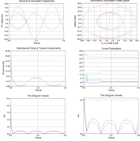

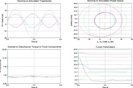

![Figure A.4.3. Simulation results for “slow” motion Ω =5 [rad/s] without (LHS) and with (RHS) external perturbation using only the Symplectizing Algorithm: the norm of the “truncated generalized force components” (1 st row) and the generalized forces](https://thumb-eu.123doks.com/thumbv2/9dokorg/1278685.101838/108.892.115.715.452.841/simulation-perturbation-symplectizing-algorithm-truncated-generalized-components-generalized.webp)
![Figure A.4.5. Simulation results for “normal” motion Ω =10 [rad/s] without (LHS) and with (RHS) external perturbation (1 st row) and the variation of the tuned](https://thumb-eu.123doks.com/thumbv2/9dokorg/1278685.101838/110.892.116.718.353.938/figure-simulation-results-normal-motion-external-perturbation-variation.webp)
![Figure A.4.7. Simulation results for “very fast” motion Ω =25 [rad/s], without (LHS) and with (RHS) external perturbation without complementary tuning (the first two rows) and with complementary tuning of step length 10 -5 [dimensionless] (3 rd and 4](https://thumb-eu.123doks.com/thumbv2/9dokorg/1278685.101838/112.892.116.722.99.886/figure-simulation-results-external-perturbation-complementary-complementary-dimensionless.webp)

