H
∞control of nonlinear systems with positive input with application to
antiangiogenic therapy ?
D´aniel A. Drexler∗ Johanna S´api∗ Levente Kov´acs∗
∗Physiological Controls Research Center, University Research, Innovation and Service Center, ´Obuda University, Hungary (e-mails:
{drexler.daniel,sapi.johanna,levente.kovacs}@nik.uni-obuda.hu).
Abstract:
There are many systems in practice that can have only positive (nonnegative) input, typical examples for such systems are physiological systems. Moreover, the parameters of these systems are usually not known exactly or may vary over time, thus application of robust controllers represents a reasonable possibility. Most model-based controller design methods are developed for systems that can (or must) have negative and positive inputs as well, thus a dynamical extension is given here to the original system that ensures that the input of the original system is positive but the extended system can have negative input as well. The current paper investigates a robust control design method with positive input for an automatic therapy possibility in the case of antiangiogenic targeted molecular therapy using a recently published tumor growth model based on mice experiments. The extended system is transformed into an integrator series that is further modified using state-feedback to prepare the system for H∞norm-based controller synthesis. The simulations demonstrate the robustness of the controller and the positivity of the input.
Keywords:Positive systems, Robust control, Output feedback control, Biomedical system modeling and simulation, Decision support and control
1. INTRODUCTION
Positive systems form a relevant subset of dynamic systems (Haddad et al. (2010)). The domain of positive (or non- negative) systems is constrained onto the positive orthant, and the input of positive systems is typically constrained to be positive as well. However, most model-based control design methods are developed for systems whose input can have any sign, thus they can not incorporate the constraint imposed on the input.
Most physiological systems are positive systems, consider e.g. blood-glucose regulatory system models (Yu et al.
(2018), Misgeld et al. (2018)), tumor growth models (Hah- nfeldt et al. (1999), d’Onofrio and Gandolfi (2004), S´api et al. (2017), Ferenci et al. (2017), Drexler et al. (2017b)) or chemical reactions (Drexler et al. (2018)). Control of these systems can be difficult due to the constraint that their input most be positive. Moreover, these systems typically have uncertain parameters or parameters whose value vary over time, thus application of robust control methodologies may become necessary.
Robust control of physiological systems have already been considered in the literature by many authors, see e.g. Malagutti et al. (2013), Ahmed and ¨Ozbay (2015), Colmegna et al. (2016), Colmegna et al. (2018) , Kov´acs
? This project has received funding from the European Research Council (ERC) under the European Union’s Horizon 2020 research and innovation programme (grant agreement No 679681).
(2017) or Kov´acs et al. (2014). However, positivity of the input has not been considered as an issue during controller design. Positivity of the input has been considered e.g. in Kov´acs et al. (2014) by adding a saturation at the con- troller output, which is not considered during the design phase.
In Drexler et al. (2017c,d) positivity of the input has been incorporated into the control design process. The model of the plant has been extended with the differential equation of the input that is defined as a bilinear equation of the original system input, and a new, fictive system input. This system is positive, thus the original input is positive for any values of the fictive input as it is shown in Subsection 2.1. As a result, one can design a controller for the extended system that gives the control law for the fictive input, and the positivity of the original input will be guaranteed by the dynamic extension.
However, as a result of the dynamic extension that ensures positive input for the original system, the extended system will be nonlinear even if the original system was linear. In Drexler et al. (2017c,d) the extended systems are linearized using feedback linearization, and path tracking control is applied. However, feedback linearization (discussed in Subsection 2.2) transforms the system into a series of integrators that have infinite H∞ norm, which is not suitable for H∞ norm-based controller design. Our aim is to design a robust controller with positive input based
on H∞ norm, thus the series of integrators form is not desirable.
The feedback linearized system is transformed to a linear system with prescribed (nonzero) poles and static gain of one in Subsection 3.1. This system is now suitable for robust control design. The applied system interconnection structure and robust control design method is given in Subsection 3.2.
The positive input robust control design methodology is applied to a tumor growth model under the effect of an antiangiogenic drug given in Drexler et al. (2017a) validated using mice experiments. The resulting controller is validated using simulations in Section 4 with ±20%
variation in relevant tumor growth parameters (tumor cell division rate and the drug efficiency). The simulation results show that the positivity of the input is maintained and the closed-loop system is robust against parametric variations.
2. POSITIVE CONTROL AND LINEARIZATION Consider a nonlinear, smooth, input affine system with dynamics described by
˙
x=f(x) +g(x)u (1)
withx∈ C∞(R,Rn),u∈ L∞(R,R),f ∈ C∞(Rn,Rn), and g∈ C∞(Rn,Rn). Let the output of the system be given by
y=h(x) (2)
with y ∈ C∞(R,R) and h ∈ C∞(Rn,R). Moreover, we suppose that the input must be nonnegative, i.e.u(t)≥0 for every t∈R.
2.1 Positive control
In order to guarantee the positivity of the input, we extend the system with the dynamics
˙
u=−uv (3)
wherev∈ L∞(R,R). The solution to (3) for allt≥0 with initial conditionu(0) is
u(t) =u(0) exp
−
t
Z
0
v(τ)dτ
. (4) Ifu(0)>0, then the solution is always positive, regardless of the functionv. Consider the extended system with the new fictive inputv and the extended state vector
˜ x=
x u
(5) whose dynamics is described by the differential equation
x˙
˙ u
| {z }
˜˙ x
=
f(x) +g(x)u 0
| {z }
f(˜˜x)
+ 0
−u
| {z }
˜ g(˜x)
v. (6)
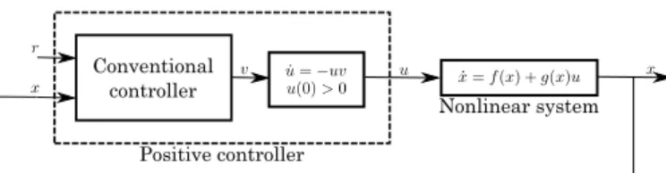
If the controller is applied for the extended system, and the controller defines the control law for the fictive input v, the dynamical extension will guarantee that the real system input (u) will be positive (Drexler et al. (2017c,d)).
Thus, the controller is designed for the extended system;
however the dynamical extension is implemented in the controller (Fig. 1).
Conventional controller
Positive controller
Nonlinear system
Fig. 1. Controller architecture with positive input dynam- ics extension
2.2 Feedback linearization
The extended system is a nonlinear system even if the original system was linear, due to the nonlinear dynamics (3). Thus, we linearize the system using state feedback (Isidori (1995)).
Denote the Lie derivative of the scalar field h along the vector fieldf by
Lfh:=h0f, (7)
where 0 denotes differentiation with respect to the state variables, and use this notation to define recursively
Lifh:=Lf
Li−1f h
=
Li−1f h0
f (8)
withL0fh:=h. Denote the Lie derivative of the scalar field Lifhalong the vector fieldg by
LgLifh:= Lifh0
g. (9)
Using these notations, we define (point-wise) the relative degree of an outputy=h(x) as the positive integerrsuch that
LgLkfh= 0, k= 0,1, . . . , r−2 (10)
LgLr−1f h6= 0 (11)
are satisfied. The output has maximal relative degree if r=n, in this case the system (1) can be transformed into a series of integrators as
y=h (12)
˙
y=Lfh (13)
¨
y=L2fh (14)
...
y(n−1)=Ln−1f h (15)
y(n)=Lnfh+LgLn−1f hu:=w. (16) The input of the series of integrators is w, and the real input of the system is acquired using the feedback law
u= w−Lnfh LgL(n−1)f h
. (17)
Denote the states of the integrator series as z = (z1, z2, . . . , zn)>:= y,y, . . . , y˙ (n−1)>
, and the coordinate transformation between the states of the system and the states of the linear system by
Φ(x) =
h Lfh L2fh ... Ln−1f h
=z. (18)
2.3 Positive control with feedback linearization
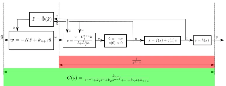
Consider the extended system (6) with positive input dynamics. Suppose that the output of the system without extension has maximal relative degree with uconsidered as the input. Then the output of the system after the dynamical extension will also have maximal relative degree withv considered as the input of the system.
The coordinate transformation between the states of the nonlinear system and the linear system are defined by
˜ z=
h Lf˜h L2˜
fh ... Ln˜
fh
:= ˜Φ(˜x) (19)
and the linearizing feedback is given by v=
w−Ln+1˜
f h
Lg˜Ln˜
fh . (20)
Note that since the order of the extended system isn+ 1, the Lie derivatives in the coordinate transformation go till the nth order, and the Lie derivatives used in the linearizing feedback are of order n+ 1.
3. H∞ NORM-BASED CONTROLLER DESIGN 3.1 Loop-shaping before controller design
The linearized system resulting after feedback linearization is composed of n+ 1 integrators, thus its H∞ norm is infinite, making the linearized system infeasible for H∞ norm-based controller design. The differential equation of the linearized system is
˙˜
z=
0 1 . . . 0 0 0 0 0 1 . . . 0 0 ... . .. ... 0 0 0 . . . 1 0 0 0 0 . . . 0 0
˜ z+
0 0 ... 0 1
w. (21)
We transform the (all zero) eigenvalues of this system to s1, s2, . . . , sn+1 such that all of them have negative real parts, by applying the state-feedback w = −Kz˜ on the linearized system, where K = (kn+1, kn, . . . , k2, k1). Let the input of the new system be denoted by ˜u. If we apply the control law w = −Kz˜+kn+1u, then the differential˜ equation of the resulting closed-loop system will be
˙˜
z=
0 1 . . . 0 0 0
0 0 1 . . . 0 0
... . .. ...
0 0 0 . . . 1 0
−kn+1 −kn −kn−1 . . . −k2 −k1
˜ z+
0 0 ... 0 kn+1
˜ u
(22) and the characteristic equation of the new system matrix is
sn+1+k1sn+k2sn−1+. . .+kn+1 (23) and the static gain of the system will be 1. Here, the feedback gain K is chosen such that the roots of (23) are the prescribed rootss1, s2, . . . , sn+1, thus the transfer function
G(s) = kn+1
sn+1+k1sn+k2sn−1+. . .+kns+kn+1
(24) of the new system will have the poless1, s2, . . . , sn+1. The H∞ norm ofG(s) is one, so it can be used as the nominal model for H∞ controller design. The architecture with positive dynamics extension, exact linearization, and pole placement is in Fig. 2.
3.2 System interconnection structure
We will apply a two degrees of freedom (2-DOF) controller (Kin Fig. 3) with control law
˜
u(s) =Kr(s)r(s)−Ky(s)y(s) (25) whereris the Laplace transform of the reference signal for the closed-loop system and y is the Laplace transform of the measured output of the system. The Laplace transform of the output of the controller is ˜u, which is the input for the linearized system in Fig 2.
The extended plant (P in Fig. 3) contains the nominal plant with transfer function G that results from the linearization in Fig. 2, the transfer functionTidthat defines the ideal transfer function of the closed-loop system, the transfer function Wn that defines the frequency content of the sensor noise, and the transfer functions Wp and Wu which define the performance of the tracking error and control input. The disturbance inputs of the extended plant P are the reference signal r and sensor noise n, the performance outputs of P are the zp and zu signals that are the filtered tracking error and control input. The control input of P is ˜u, while the measured outputs are the reference signal rand the measured system output y that is burdened with the filtered sensor noise. The system interconnection structure is shown in Fig. 3.
The closed-loop system is given by the lower fractional transformation (Zhou et al. (1996))
M =Lf(P, K); (26)
during H∞ synthesis we are searching for the controller Kthat minimizes theH∞norm of the closed-loop system M. We useγ iteration, looking for the smallest positiveγ such that the resulting controllerK will ensure that
kMk∞=kLf(P, K)k∞< γ, (27) yielding a suboptimal solution.
4. APPLICATION TO ANTIANGIOGENIC THERAPY The positive input robust controller is applied to a tumor growth model that describes the dynamics of the tumor growth under the effect of the angiogenic inhibitor called bevacizumab, and the dynamics of the inhibitor. The used model captures the core dynamics of the tumor growth and drug dynamics (i.e. tumor cell division, inhibition, drug clearance) published in Drexler et al. (2017a), with parameter values identified based on mice experiments.
For details of the experiments see S´api et al. (2015). The model is a simplified version of the the one published in Drexler et al. (2017b). The differential equations of the tumor growth model used here are
˙
x=ax−bxy (28)
˙
y=−cy+u (29)
Fig. 2. The linearization of the nonlinear system with positive input dynamics; the resulting closed-loop system with transfer functionG(s) serves as the nominal system forH∞ controller design
Fig. 3. The system interconnection structure with the extended plantP and the 2-DOF controllerK where x is the time function of tumor volumes in mm3, y is the time function of the inhibitor level in mg/kg, u is the time function of the inhibitor injection rate in mg/kg/day, a is the tumor growth rate parameter given in 1/day characterizing the speed of tumor cell division, while b is the inhibition parameter given in kg/mg/day characterizing the efficiency of the applied drug, andc is the clearance of the drug given in 1/day characterizing the speed of the depletion of the drug. The values of the
parameters are a = 0.27 1/day, b = 0.0074 kg/mg/day, andc= ln(2)/3.9 1/day (Drexler et al. (2017a)).
The tumor growth model after positive input dynamics extension is given by
˙
x=ax−bxy (30)
˙
y=−cy+u (31)
˙
u=−uv, (32)
thus the input of the extended model isv. The output of the system is the tumor volumex, soh=x, and the Lie derivatives used for feedback linearization are
Lgh= 0 (33)
LgLfh= 0 (34)
LgL2fh=bxu (35)
L3fh= ((bc−2b(a−by)) (u−cy) +. . . + (a−by)2−b(u−cy)
(a−by)
x (36) thus the system has maximal relative degree whenever x6= 0 and u6= 0, and the system is linearized using the state feedback
v= w−L3fh
bxu . (37)
The Lie derivatives used for the coordinate transformation are
Lfh=ax−bxy (38)
L2fh= (a−by)2−b(I−cy)
x (39)
thus the coordinate transformation ˜Φ is given by Φ =˜
x ax−bxy (a−by)2−b(u−cy)
x
. (40) The poles of the linearized system are transformed to
−0.5 rad/day with multiplicity of three using the feedback gain
K= ( 0.125 0.75 1.5 ) (41)
and the control law
w=−KΦ + 0.125˜˜ u. (42) The resulting system is a linear system with H∞ norm being one and transfer function G given below in (43), thus it is suitable for H∞ controller design.
The transfer functions used at the H∞ controller design are
G= 0.125
s3+ 1.5s2+ 0.75s+ 0.125 (43)
Tid= 1
(1/10)2s2+ 2(1/10)√
2/2s+ 1 (44) Wp= 10
(10s+ 1)2 (45)
Wu= 0.3 (46)
Wn= 0.1 s+ 1
0.1s+ 1. (47)
The controller design resulted in theγ value
γ= 0.9888 (48)
thus the required specifications are met by the closed-loop system.
The controller is tested using simulations that run for 300 days, with the tumor growth rate (a) and inhibition rate (b) parameters being varied by±20%. The reference signal is given as an exponential function
xref(t) =x(0) exp (−t/100) (49) with x(0) = 10000 mm3 being the initial tumor volume used in the simulations.
The resulting tumor volumes are shown in Fig. 4. In the cases when the tumor growth rate was increased by 20%, the tumor volumes initially grow, but later the tumor volumes decrease in all the cases. The tumor grows at the beginning of the treatment since the inhibitor level is very low, and due to the positive input dynamics, the inhibitor level can not change discontinuously, so the inhibitor level growth rate has a specific dynamics. After the inhibitor levels increase (see Fig. 5), the tumor regression starts.
The inhibitor levels are in Fig. 5, while the injection rates are shown in Fig. 6. The figures show that when the tumor growth rate is larger, and the inhibition rate is lower (i.e. the tumor grows faster and the effect of the inhibitor is lower), the required inhibitor dose is larger (red curve), while when the tumor growth rate is lower, and the inhibition rate is larger (i.e. when the tumor grows slower and the effect of the inhibitor is larger), the required inhibition rate is smaller (green curve), which is consistent with the expectations.
The injection rate is large at the beginning, and reaches a steady-state value after the first large injection (Fig. 6).
The initial injection is similar for all parameter values;
however, the injection rate steady-states are different, e.g.
when the tumor growth rate is larger and the inhibition rate is lower, the required inhibitor injection rate is larger (red curve). The resulted injection rate values are physi- ologically feasible, i.e. they are sufficiently low and would be appropriate for a real treatment.
0 100 200 300
0 1 2 3 4 104
a +20%
a+20%, b+20%
a+20%, b-20%
a-20%
a-20%, b+20%
a-20%, b-20%
Fig. 4. The simulated tumor volumes in the closed-loop with perturbation of the model parametersaandb
0 100 200 300
0 20 40 60
80 a +20%
a+20%, b+20%
a+20%, b-20%
a-20%
a-20%, b+20%
a-20%, b-20%
Fig. 5. The simulated inhibitor levels in the closed-loop with perturbation of the model parametersaandb
0 100 200 300
0 5 10 15
a +20%
a+20%, b+20%
a+20%, b-20%
a-20%
a-20%, b+20%
a-20%, b-20%
Fig. 6. The simulated injection rates in the closed-loop with perturbation of the model parametersaandb
5. CONCLUSION
The positive input dynamics methodology was further developed such that the positive system is transformed into a linear system that can be used forH∞ norm-based robust controller design. The design methodology has been applied to a tumor growth model, and simulations have shown that the developed methodology is suitable to de- sign robust controller with guaranteed positive controller output.
The original system is nonlinear, which is linearized us- ing exact linearization. Exact linearization is not robust, since it is based on exact cancellation of nonlinear terms.
However, simulations have shown that with application of the dynamic extension and the linear transformation be- sides exact linearization, the closed-loop system is robust against parametric perturbations, moreover, the positivity of the input is guaranteed all the time.
ACKNOWLEDGEMENTS
The present work has partially been supported by the Hungarian National Research, Development and Innova- tion Office (TT 16 1-2016-0070 and SNN 125739).
REFERENCES
Ahmed, S. and Ozbay, H. (2015).¨ Switching ro- bust controllers for automatic regulation of postop- erative hypertension using vasodilator drug infusion rate. IFAC-PapersOnLine, 48(26), 224 – 229. doi:
https://doi.org/10.1016/j.ifacol.2015.11.141.
Colmegna, P., S´anchez-Pe˜na, R., and Gondhalekar, R.
(2018). Linear parameter-varying model to design control laws for an artificial pancreas. Biomedical Signal Processing and Control, 40, 204 – 213. doi:
https://doi.org/10.1016/j.bspc.2017.09.021.
Colmegna, P.H., S´anchez-Pe˜na, R.S., Gondhalekar, R., Dassau, E., and Doyle, F.J. (2016). Switched lpv glucose control in type 1 diabetes. IEEE Transactions on Biomedical Engineering, 63(6), 1192–1200. doi:
10.1109/TBME.2015.2487043.
d’Onofrio, A. and Gandolfi, A. (2004). Tumor eradication by antiangiogenic therapy: analysis and extensions of the model by hahnfeldt et al. (1999). Mathematical Biosciences, 191(2), 159–184.
Drexler, D.A., S´api, J., and Kov´acs, L. (2017a). A minimal model of tumor growth with angiogenic inhibition using bevacizumab. InProceedings of the 2017 IEEE 15th In- ternational Symposium on Applied Machine Intelligence and Informatics, 185–190.
Drexler, D.A., S´api, J., and Kov´acs, L. (2017b). Modeling of tumor growth incorporating the effects of necrosis and the effect of bevacizumab. Complexity, 1–10. doi:
10.1155/2017/5985031.
Drexler, D.A., S´api, J., and Kov´acs, L. (2017c). Positive control of a minimal model of tumor growth with be- vacizumab treatment. In Proceedings of the 12th IEEE Conference on Industrial Electronics and Applications, 2081–2084.
Drexler, D.A., S´api, J., and Kov´acs, L. (2017d). Positive nonlinear control of tumor growth using angiogenic inhibition. IFAC-PapersOnLine, 50(1), 15068 – 15073.
doi:https://doi.org/10.1016/j.ifacol.2017.08.2522. 20th IFAC World Congress.
Drexler, D.A., Vir´agh, E., and T´oth, J. (2018). Control- lability and reachability of reactions with temperature and inflow control.Fuel, 211(Supplement C), 906 – 911.
doi:https://doi.org/10.1016/j.fuel.2017.09.095.
Ferenci, T., S´api, J., and Kov´acs, L. (2017). Modelling tumor growth under angiogenesis inhibition with mixed- effects models.Acta Polytechnica Hungarica, 14(1), 221–
234.
Haddad, W.M., Chellaboina, V., and Hui, Q. (2010).
Nonnegative and Compartmental Dynamical Systems.
Princeton University Press.
Hahnfeldt, P., Panigrahy, D., Folkman, J., and Hlatky, L.
(1999). Tumor development under angiogenic signal- ing: A dynamical theory of tumor growth, treatment response, and postvascular dormancy.Cancer Research, 59, 4770–4775.
Isidori, A. (1995). Nonlinear Control Systems. Springer- Verlag London.
Kov´acs, L. (2017). Linear parameter varying (lpv) based robust control of type-i diabetes driven for real patient data. Knowledge-Based Systems, 122, 199 – 213. doi:
https://doi.org/10.1016/j.knosys.2017.02.008.
Kov´acs, L., Szeles, A., S´api, J., Drexler, D.A., Rudas, I., Harmati, I., and S´api, Z. (2014). Model-based angio- genic inhibition of tumor growth using modern robust control method. Computer Methods and Programs in Biomedicine, 114, e98–e110.
Malagutti, N., Dehghani, A., and Kennedy, R.A. (2013).
Robust control design for automatic regulation of blood pressure. IET Control Theory Applications, 7(3), 387–
396. doi:10.1049/iet-cta.2012.0254.
Misgeld, B.J., Tenbrock, P.G., Dassau, E., Doyle, F., and Leonhardt, S. (2018). Optimal online selection of type 1 diabetes-glucose metabolism models. Control Engineering Practice, 71(Supplement C), 108 – 119. doi:
https://doi.org/10.1016/j.conengprac.2017.10.007.
S´api, J., Kov´acs, L., Drexler, D.A., Kocsis, P., Gaj´ari, D., and S´api, Z. (2015). Tumor volume estimation and quasi-continuous administration for most effective bevacizumab therapy. PLoS ONE, 10(11), 1–20. doi:
10.1371/journal.pone.0142190.
S´api, J., Drexler, D.A., and Kov´acs, L. (2017). Poten- tial benefits of discrete-time controller-based treatments over protocol-based cancer therapies.Acta Polytechnica Hungarica, 14(1), 11–23.
Yu, X., Turksoy, K., Rashid, M., Feng, J., Hobbs, N., Hajizadeh, I., Samadi, S., Sevil, M., Lazaro, C., Mal- oney, Z., Littlejohn, E., Quinn, L., and Cinar, A. (2018).
Model-fusion-based online glucose concentration predic- tions in people with type 1 diabetes. Control Engi- neering Practice, 71(Supplement C), 129 – 141. doi:
https://doi.org/10.1016/j.conengprac.2017.10.013.
Zhou, K., Doyle, J.C., and Glover, K. (1996). Robust and Optimal Control. Prentice-Hall, Inc., Upper Saddle River, NJ, USA.