Improved High Dynamic Range Image Reproduction Method

Improved High Dynamic Range Image Reproduction Method

András Rövid

, Takeshi Hashimoto

1 Department of Vehicles and Light-Weight Structure Analysis Budapest University of Technology and Economics

Bertalan Lajos u. 2, H-1111 Budapest, Hungary e-mail: rovid@kme.bme.hu

1, 2

Department of Electrical and Electronics Engineering, Shizuoka University 5-1, 3-chome Johoku, Hamamatsu, 432-8561, Japan

e-mail: tethash@ipc.shizuoka.ac.jp

Abstract: High dynamic range (HDR) of illumination may cause serious distortions and other problems in viewing and further processing of digital images. This paper describes a new algorithm for HDR image creation based on merging images taken with different exposure time. There are many fields, in which HDR images can be used advantageously, with the help of them the accuracy, reliability and many other features of the certain image processing methods can be improved.

Keywords: high dynamic range, multiple exposures, segmentation

1 Introduction

Digital processing can often improve the visual quality of real world photographs, even if they have been taken with the best cameras by professional photographers in carefully controlled lighting conditions. This is because visual quality is not the same thing as accurate scene reproduction. In image processing most of the recently used methods apply a so called preprocessing procedure to obtain images which guarantees – from the point of view of the concrete method – better conditions for the processing. Eliminating noise from the images yields much better results as else.

There are many kinds of image properties to which the certain methods are more or less sensitive [1] [2]. Certain image regions have different features. The parameters of the processing methods in many cases are functions of the image features. The light intensity at a point in the image is the product of the reflectance at the corresponding object point and the intensity of illumination at that point.

The amount of light projected to the eyes (luminance) is determined by factors such as: the illumination that strikes visible surfaces, the proportion of light reflected from the surface and the amount of light absorbed, reflected or deflected by the prevailing atmospheric conditions such as haze or other partially transparent media [3]. An organism needs to know about meaningful world properties, such as color, size, shape, etc. These properties are not explicitly available in the retinal image and must be extracted by visual processing. In this paper we will deal with the reproduction of the image when the high dynamic range of the lightness causes distortions in the appearance and contrast of the image in certain regions e.g. because a part of the image is highly illuminated looking plain white or another is in darkness. High dynamic range (HDR) images enable to record a wider range of tonal detail than the cameras could capture in a single photo.

Dynamic range in photography describes the ratio between the maximum and minimum measurable light intensities. HDR imaging is a set of techniques that allow a far greater dynamic range of exposures than normal digital imaging techniques [4]. HDR capable sensors play an important role in the traffic safety as well, therefore they are important for use with cars because they must operate in dark and bright environments. An HDR sensor, in contrast to a linear sensor, can detect details that bright environments wash out, and it misses fewer details in dark environments [4]. Using HDR techniques in preprocessing phase of the images, the performance of different image processing algorithms can be improved, e.g. corner and edge detectors.

The paper is organized as follows: Section II gives a short overview of the existing principles, Section III describes the basic concept of the algorithm, Section IV introduces the so called detail factor and its estimation, while Section V describes the proposed method more detailed and finally Section VI and Section VII report conclusions and experimental results.

2 Background

There are some existing methods, which main aim is to obtain as detailed image as possible from multiple exposures. For example method in [5] is based on fusion in the Laplacian pyramid domain. The core of the algorithm is a simple maximization process in the Laplacian domain. Wide dynamic range CMOS image sensors play also very important role in HDR imaging [6]. The sensor introduced in [6] uses multiple time signals and such a way extends the dynamic range of the image sensor.

3 The Basic Concept

If the scene contains regions with high luminance values, then to see the details in that highly illuminated regions it is necessary to take a picture with lower exposure time, on the other hand if the scene contains very dark areas, then this exposure time should be higher. In such cases taking just only one image is not enough to capture every detail of the scene, more pictures are needed with various exposure time.

Given N images of the same scene, which were taken using different exposure time. The proposed method combines the given N images into a single HDR image in which each of detail involved in the input images can be found. The main idea of the method is the following. First of all, it is necessary to detect those regions of the input images in which the level of the involved detail is larger then the level of the same region in the other N-1 images. This procedure is performed by segmenting the images into small rectangular regions of the same size. One region can contain many but a limited number of connected local rectangular areas. The output HDR image is obtained by merging the estimated regions together. By the merging not just the contents of the regions have to be merged, but the sharp transitions, which occur between the borders of the regions should be also eliminated. For this purpose smoothing functions can be used. In this paper the Gaussian hump is used as the smoothing function. To each region one Gaussian function is assigned, with center coordinates identical to the center of gravity of the corresponding region. Finally, using the obtained regions and the corresponding Gaussian, blending procedure is applied to obtain the resulted HDR image. The quality of the output can be influenced by several parameters, like the size of the regions, the parameters of the Gaussian and the size of the rectangular areas, which were mentioned at the beginning of this section.

4 Measuring the Level of the Detail in an Image Region

For extracting all of the details involved in a set of images of the same scene made with different exposures, it is required to introduce a factor for characterizing the level of the detail in an image region. For this purpose the gradient of the intensity function was used, corresponding to the processed image and a linear mapping function, which was applied for setting up the sensitivity of the measurement of the detail level. In the followings the description of the estimation of the mentioned factor is introduced.

Let I(x, y) be the pixel luminance at location [x, y] in the image to be processed.

Let us consider the group of neighboring pixels which belong to a 3×3 window

centered on [x, y]. For calculating the gradient of the intensity function in horizontal Ix and vertical Iy directions at position [x, y] the luminance differences between the neighboring pixels were used:

(x 1,y) ( )I x,y , I

I_x= + −

Δ (1)

(x,y 1) ( )I x,y . I

I_y = − −

Δ (2)

For the further processing the maximum of the estimated gradient values should be chosen, which solves as the input of the linear mapping function P defined as follows:

( )v v/I_max,

P = (3)

where Imax is the maximal luminance value. For 8 bit grayscale images it equals 255. Let R be a rectangular image region of width rw and height rh, with upper left corner at position [xr, yr]. The level of the detail inside of the region R can be defined as follows:

( )

( )

0 0

∑∑

= ^{rw h}

i r

j ij

h w

e

D Pr

r r

M R N (4)

where rij stands for the maximum of the gradients in horizontal and vertical direction [1], i.e.

( ) ( )

(

)

max I x i y j I x i y j

r_ij= Δ _{x r}+ _r+ Δ _{y r}+ _r+ (5)

and Ne represents the number of pixel positions inside the region R for which rij >

0. As higher is the calculated MD value, as detailed is the analyzed region. In the followings we will use this parameter for characterizing the measure of the image detail.

5 Description of the Algorithm for Measuring the Level of the Detail in an Image Region

Let Ik denote the intensity function of the input image with index k, where k=1..N and N stands for the number of images to be processed, each of them taken with different exposure time. Each image contains regions, which are more detailed as the corresponding regions in the other N-1 images. Our goal is to produce an image, which is the combination of the input N images and contains all details involved in them without producing noise. Using such detailed image, the most of the feature detection methods can be improved and can effectively be used even if the lighting conditions are not ideal. The first step of the processing is to divide the pictures into small rectangular areas of same size. Let w×h be the size of these areas, where w is the width and h the height of the rectangular area (see Fig. 1).

Figure 1

Illustration of the certain exposures and the small rectangles, inside of which the detail factor is estimated

After this division a grid of size nxm is obtained for each input image, where n and m represent the number of rectangular areas in horizontal and vertical direction respectively.

Let aijk be the area in the ith row and jth column of the grid corresponding to the image with index k (see Fig. 1). Let D be the matrix of highest detail factors, which element in ith row and jth column stands for the index of the image having the largest detail factor inside of the area aij among all input images (exposures), i.e.

{1,..,N} k s,s d_ij:M

( )

( )

k∈ ∧ ≠ = _D ≥ _D

∀ (6)

where dij stands for the element in the ith row and jth column of matrix D. Now, we have the matrix D, which contains the indices of the input images with largest detail factor corresponding to the certain rectangular areas. Using this matrix we can easily find the areas with largest detail factor and merge them together. If we take into account the processing time necessary for such merging – which involves also the smoothing process for eliminating the sharp should be reduced to obtain the output in a desirable time interval. Increasing the size of the rectangular areas reduces the processing time, but the quality of the resulted HDR image will be lower. The reason is that large rectangular areas can fall with high probability onto such image positions, where a part of a concrete area can contain very detailed and non-detailed subareas, as well.

In the followings we will describe how to avoid such effects and how to increase the processing time by maintaining the quality of the output. As solution we can create a predefined number of groups using the small rectangular areas. By the creation the distance between the centers of the areas with the highest detail level corresponding to the same input image is used.

Figure 2

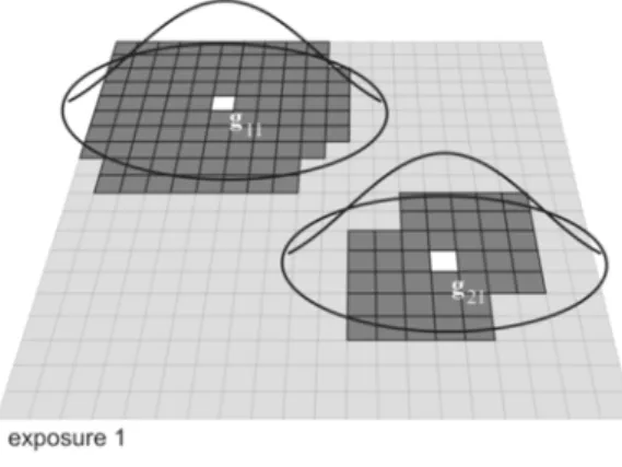
Illustration of the groups and their centers of gravities (black and dark gray rectangles). The figure illustrates a situation when two input images are given. The white region represents those areas of the first input image, which have the largest detail factor comparing to the same area in the second image.

On the other hand the gray region illustrates those areas, which detail factor is the largest comparing to the same area in the first image

Figure 3

Illustration of an image segmented into groups. The dark gray areas are those which detail factor is the largest among all images. The white squares are illustrating the centers of gravities corresponding to

the certain groups. Furthermore the Gaussian humps centered at gij positions can be seen. The small rectangles are the areas aij.

There is a lot of different series of such groups. We can form a group for example as follows: Suppose that we want to group those areas of the input image with index k, for which dij=k. First we take an arbitrary area aij satisfying the equation dij=k as the first element of a group.

As next step we are searching for such areas and add them to this group, which distance to the center of the first element of the group is below a predefined threshold value. If there are no other areas then we can form another group from the remaining areas using the same procedure.

Figure 4

Illustrating a similar situation like in Fig. 3, but in this case the exposure 2 can be seen

Finally a set of groups is obtained, which centers of gravity are uniformly distributed among the areas of the kth image satisfying the equation dij=k. The whole process is repeated for each input image. An illustration of the result is shown in Fig. 2.

Let Lk be the number of the created groups of the input image with index k=1..N and let gpk = [gpkx, gpky] denote the horizontal and vertical coordinate of the center of gravity of the pth group of the image with index k, where p = 1..Lk (see Fig. 3- 4). By the merging we will use the fuzzy theory in combination with the blending functions and theory [7][8][9][10]. First we have to choose a function, which is continuous and differentiable (C¹, C²). Furthermore this function should have the maximal value at an estimated center of gravity gpk, and is decreasing proportional to the distance to gpk. These requirements are fulfilled for example by the Gaussian hump. If we place a Gaussian function over each gpk position, we can combine the certain groups of each image without producing sharp borders between the transitions. Before combining the groups, so called membership functions have to be constructed having the following properties.

( ), 1,

1 1

∑∑

= =

N k

L

p pk

k μ x y (7)

where µpk stands for the membership function corresponding to the group with center of gravity gpk. In other words, using the membership functions, we can calculate the membership values of an arbitrary pixel position in the estimated groups. We can refer to these groups also as fuzzy sets [7]. Taking into account the above described conditions and requirements, the membership values pk can be defined as follows [10]:

( )

( ) ( )

( ) ( ) ,

,

1 1

2 2

2 2

2 2 2

2 2

2 2

2

∑∑

⎟⎟

⎠

⎞

⎜⎜

⎝

⎛ −

− +

−

⎟⎟

⎠

⎞

⎜⎜

⎝

⎛ −

− +

−

=

N u

L v

g g y x

g y g x

pk

u

y vuy x vux

y pky x pkx

e y e

x

σ σ

σ σ

μ (8)

where p and k represent the group index and the input image index respectively, σx

and σy stand for the standard deviation of the Gaussian function. Let Gpk describe the group or fuzzy set with center of gravity gpk. Now we know the fuzzy sets and their membership functions. The next step is to construct the so called fuzzy rules of the form:

IF (x is from A) THEN y = B.

The meaning of this structure is the following: If the element x is the member of fuzzy set A with a non-zero membership value then the output value y is from fuzzy set B with a membership proportional to the membership value of the element x in fuzzy set A. In our case a fuzzy set Gpk will correspond to fuzzy set A, y to the output intensity and B to the intensity function of the images corresponding to Gpk. Our fuzzy rules have the following form:

IF (q is from G11) THEN Iout = I1

IF (q is from G21) THEN Iout = I1

...

IF (q is from _,1

L1

G ) THEN Iout = I1

IF (q is from G12) THEN Iout = I2

IF (q is from G22) THEN Iout = I2

...

IF (q is from ₂

L2

G ) THEN Iout = I2

. . .

IF (q is from G1N) THEN Iout = IN

IF (q is from G2N) THEN Iout = IN

...

IF (q is from _{L N}

GN ) THEN Iout = IN

where q = (x, y) is an arbitrary point in the image domain and Iout stands for the intensity of the output pixel at location q. After evaluation of the fuzzy rules the output can be written as follows:

( ), ( ) ( ), , .

1 1

∑∑

= ^N

k L

p pk k

out

k x yI x y

y x

I μ

(9) The output luminance can be influenced by changing the threshold for the distance between the centers of the areas, i.e. the size of the groups. The standard deviation also enables to influence the output HDR image. As smaller is the standard deviation as higher influence the regions have with low detail level onto the result.

Using such detailed image the edges can be also effectively extracted and advantageously used by further processing, e.g. object recognition, scene reconstruction, etc.

Conclusions

In this paper a new gradient based approach for extracting the image details was introduced, which is using multiple exposure images of the same scene as input data. The image parts involving the highest detail are choosen from each input image. Finally these parts are blended together using Gaussian blending functions.

The proposed method can be applied for color images, as well. In this case the whole procedure for each color component has to be applied. As result a HDR image is obtained. The method can advantageously be applied, when the luminance properties are not appropriate, and each detail of the scene can not be captured using one exposure time only.

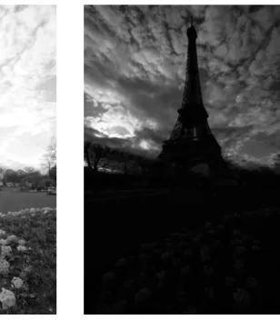
Examples

In this example the width and the height of the rectangular areas was chosen to be 5 pixels. Deviations σx=120 and σy=120 in this example. In Figs. 5 and 6 an overexposed and an underexposed image can be seen. Fig. 7 represents the resulted HDR images using the proposed method.

Acknowledgement

This work was supported by the Hungarian National Science Research Found (OTKA) under grants T048756 and T042896.

References

[1] F. Russo, “Fuzzy Filtering of Noisy Sensor Data,” in In Proc. of the IEEE Instrumentation and Measurement Technology Conference, Brussels, Belgium, 4-6 June 1996, pp. 1281-1285

[2] F. Russo, “Recent Advances in Fuzzy Techniques for Image Enhancement,” IEEE Transactions on Instrumentation and Measurement, 1998, Vol. 47, No. 6, pp. 1428-1434

[3] E. Adelson, A. Pentland, “The Perception of Shading and Reflectance,” in In D. Knill and W. Richards (eds.), Perception as Bayesian Inference, New York: Cambridge University Press, 1996, pp. 409-423

Figure 5 The input overexposed image

Figure 6

The input underexposed image

Figure 7

The resulted image after applying the proposed method

[4] L. S. Y. Li, E. Adelson, “Perceptually-based Range Compression for High Dynamic Range Images,” Journal of Vision, 2005, Vol. 5, No. 8, p. 598 [5] A. B. R. Rubinstein, “Fusion of Differently Exposed Images,” in Final

Project Report, Israel Institute of Technology, 2004, p. 14

[6] S. K. Y. W. M. Sasaki, M. Mase, “A Wide Dynamic Range Cmos Image Sensor with Multiple Exposure Time Signals and Column-Parallel Cyclic a/d Converters,” in IEEE Workshop on Charge-Coupled Devices and Advanced Image Sensors, 2005

[7] B. Y. George J. Klir, “Fuzzy Sets and Fuzzy Logic: Theory and Applications,” in Prentice Hall PTR, Munich, Germany, 1995, p. 592 [8] H. Bidasaria, “Defining and Rendering of Textured Objects through the

Use of Exponential Functions,” Graphical Models and Image Processing, 1992, Vol. 54, No. 2, pp. 97-102

[9] L. Piegl, W. Tiller, “The Nurbs Book,” in Springer-Verlag 1995-1997 (2^nd ed.), 1995, p. 646

[10] D. Breen, W. Regli, M. Peysakhov, “B-splines and Nurbs,” in Lecture, Geometric and Intelligent Computing Laboratory, Department of Computer Science, p. 42