On Robertson-type Uncertainty Principles ∗

(1)

On Robertson-type Uncertainty Principles ^∗

Attila Lovas

^†

, Attila Andai

^‡

Department for Mathematical Analysis, Budapest University of Technology and Economics,

H-1521 Budapest XI. Stoczek u. 2, Hungary August 30, 2017

Abstract

Uncertainty principles are one of the basic relations of Quantum Mechanics. Robertson has discovered first that the Schrödinger uncertainty principle can be interpreted as a determinant inequality. Generalized quantum covariance has been previously presented by Gibilisco, Hiai and Petz. Gibilisco and Isola have proved that among these covariances the usual quantum covariance introduced by Schrödinger gives the sharpest inequalities for the determinants of covariance matrices. We have introduced the concept of symmetric and antisymmetric quantumf- covariances which give better uncertainty inequalities. Furthermore, they have a direct geometric interpretation. Using a simple matrix analytical framework, we present here a short and tractable proof for the celebrated Robertson uncertainty principle.

Introduction

In quantum information theory, the most popular model of the quantum event algebra associated to ann-level system is the projection lattice of an n-dimensional Hilbert space (L(Cⁿ)). According to Gleason’s theorem [2], forn >2the states are of the form

(∀P ∈ L(Cⁿ)) P 7→Tr(DP),

whereDis a positive semidefinite matrix with trace1hence the quantum mechanical state space arises as the intersection of the standard cone of positive semidefinite matrices and the hyperplane of trace one matrices. Let us denote byMnthe set ofn×npositive definite matrices and byM¹_nthe interior of then-level quantum mechanical state space, namelyM¹_n ={D∈ Mn|TrD= 1, D >0}. LetM_n,sa be the set of observables of then-level quantum system, in other words the set ofn×nself adjoint matrices, andMn,sa⁽⁰⁾ stands for the set observables with zero trace. Observables are non commutative analogues of random variables known from Kolmogorovian probability. If A is an observable, then the expectation ofAin D∈ M¹_n is defined byED(A) = Tr(AD).

Spaces Mn and M¹_n are form convex sets in the space of self adjoint matrices, and they are obviously differentiable manifolds [7]. The tangent space ofMn at a given stateD can be identified withM_n,saand the tangent space ofM¹_n withMn,sa⁽⁰⁾ . Monotone metrics are the quantum analogues of the Fisher information matrix known from classical information geometry. Petz’s classification

∗keywords: uncertainty principle, quantum Fisher information, quantum information geometry; MSC: 62B10, 94A17

†lovas@math.bme.hu

‡andaia@math.bme.hu

(2)

theorem [11] establishes a connection between monotone metrics and the set of symmetric and normalized operator monotone functions F_op. For the mean induced by the operator monotone functionf ∈ Fop we also introduce the notation

mf :R⁺×R⁺ →R⁺ (x, y)7→yf x

y

.

The monotone metric associated tof ∈ Fop is given by

K_D⁽ⁿ⁾(X, Y) = Tr

Xm_f(L_n,D, R_n,D)⁻¹(Y)

for alln∈NwhereLn,D(X) =DX,Rn,D(X) =XDfor allD, X∈Mn(C). The metricK_D⁽ⁿ⁾can be extended to the spaceMn. For every D∈ Mn and matricesA, B∈M_n,sa let us define

hA, Bi_D,f = Tr

Amf(Ln,D, Rn,D)⁻¹(B) ,

with this notion the pair (Mn,h·,·i_·,f)will be a Riemannian manifold for every operator monotone functionf ∈ Fop.

Although the generalization of expectation and variance to the non commutative case is straightforward, covariance has many different possible generalization to the quantum case.

Schrödinger has defined the (symmetric) covariance of the observables for a given stateD as

CovD(A, B) = 1

2(Tr(DAB) + Tr(DBA))−Tr(DA) Tr(DB).

In a recent paper [9], we have introduced the concept ofsymmetricf-covarianceas the scalar product of anti-commutators

qCov^s_D,f(A, B) =f(0)

2 h{D, A},{D, B}i_D,f.

Note that, qCov^s_D,f(A, B)coincides with CovD(A, B) wheneverf(x) = ^1+x₂ . We have proved that for anyf symmetric and normalized operator monotone function

det

f(0)

2 h{D, Ah},{D, Aj}i_D,f

h,j=1,...,N

!

≥det

f(0)

2 hi [D, Ah],i [D, Aj]i_D,f

h,j=1,...,N

!

(1) eq:introfirstresult

holds. Moreover we showed that the function f0(x) = ¹₂

1+x

2 +_1+x^2x

gives the smallest universal upper bound for the right-hand side, that is, for every symmetric and normalized operator monotone functiong

det

f0(0)

2 h{D, A_h},{D, A_j}i_D,f

0

h,j=1,...,N

!

≥det g(0)

2 hi [D, A_h],i [D, A_j]i_D,g

h,j=1,...,N

!

(2) eq:introsecondresult

holds.

The Equations (1) and (2) are Robertson-type uncertainty principles with clear geometric meaning, namely, they can be viewed as a kind of volume inequalities. The volume of the N-parallelotope spanned by the vectorsX_k (k= 1, . . . , N) with respect to the inner product h·,·iis

V_f(X₁, . . . , X_N) = s

det h

hX_h, X_ji_D,fi

h,j=1,...,N

.

(3)

In this setting Equation (1) and (2) can be written as

V_f({D, A₁}, . . . ,{D, A_N})≥V_f(i [D, A₁], . . . ,i [D, A_N]) Vf₀({D, A1}, . . . ,{D, AN})≥Vg(i [D, A1], . . . ,i [D, AN]).

To make the explanation self contained and understandable for the largest possible audience, in Section 1, we briefly outline the origin and development of Robertson-type uncertainty principles. In Section 2, we present a simple and rather understandable proof for the original Robertson uncertainty principle.

1 Overview

The concept of uncertainty was introduced by Heisenberg in 1927 [6], who demonstrated the impossibility of simultaneous measurement of position (q) and momentum (p). He considered Gaussian distributions (f(q)), and defined uncertainty offas its widthDf. If the width of the Fourier transform off is denoted byD_F(f), then the first formalisation of the uncertainty principle can be written as

D_fD_F(f)=constant.

In 1927 Kennard generalised Heisenberg’s result [8], he proved the inequality

Var_D(A) Var_D(B)≥ 1 4

for observables A, B which satisfy the relation [A, B] = −i, for every state D, where Var_D(A) = Tr(DA²)−(Tr(DA))².

In 1929 Robertson [12] extended Kennard’s result for arbitrary two observablesA, B

VarD(A) VarD(B)≥1

4|Tr(D[A, B])|².

In 1930 Scrödinger [14] improved this relation including the correlation between observablesA, B

VarD(A) VarD(B)−CovD(A, B)²≥ 1

4|Tr(D[A, B])|². The Schrödinger uncertainty principle can be formulated as

det

CovD(A, A) CovD(A, B) Cov_D(B, A) Cov_D(B, B)

≥det

−i 2

Tr(D[A, A]) Tr(D[A, B]) Tr(D[B, A]) Tr(D[B, B])

.

For the set of observables(Ai)1,...,N this inequality was generalised by Robertson in 1934 [13] as

det

[CovD(Ah, Aj)]h,j=1,...,N

≥det

−i

2Tr(D[Ah, Aj])

h,j=1,...,N

! .

The main drawback of this inequality is that the right-hand side is identical to zero wheneverN is odd.

Gibilisco and Isola in 2006 conjectured that

det

≥det

f(0)

2 hi [D, Ah],i [D, Aj]i_D,f

h,j=1,...,N

!

, (3) eq:GibiliscoConjecture

(4)

holds [5], where the scalar producth·,·i_D,f is induced by an operator monotone functionf, according to Petz classification theorem [11]. We note that if the density matrix is not strictly positive, then the scalar product h·,·i_D,f is not defined. For arbitrary N the conjecture was proved by Andai [1]

and Gibilisco, Imparato and Isola [4]. The inequality (3) is calleddynamical uncertainty principle [3]

because the right-hand side can be interpreted as the volume of a parallelepiped determined by the tangent vectors of the time-dependent observablesAk(t) = eⁱ^tDAke⁻ⁱ^tD.

Gibilisco, Hiai and Petz studied the behaviour of a possible generalization of the covariance under coarse graining and they deduced that the covariance must have the following form for traceless observablesA, B

Cov^f_D(A, B) = Tr

Af(Ln,DR⁻¹_n,D)Rn,D(B)

, (4) petzcov

whereL_n,DandR_n,Dare superoperators acting onn×nmatrices likeL_n,D(A) =DA,R_n,D(A) =AD and f is a symmetric and normalized operator monotone function [3]. Quantum covariances of the form (4) are called quantum f-covariance, which has been introduced for the first time by D. Petz [10]. It has been proved [3] that the generalized form of dynamical uncertainty principle holds true for an arbitrary quantumf-covariance

det

[Cov^g_D(Ah, Aj)]h,j=1,...,N

≥det h

f(0)g(0)hi [D, Ah],i [D, Aj]i_D,fi

h,j=1,...,N

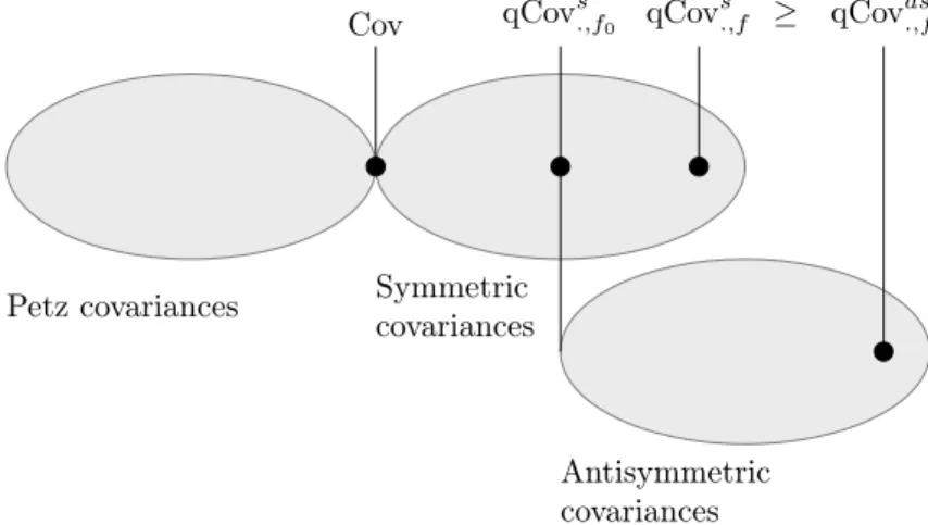
and for allgsymmetric and normalized operator monotone function. Ifg(x) = ^1+x₂ is chosen, then we get the sharpest form of the inequality. Uncertainty relations involving different type of covariances are illustrated in Figure 1.

Petz covariances Symmetric covariances

Antisymmetric covariances

Cov qCov^s_.,f₀ qCov^s_.,f ≥ qCov^as_.,f

Figure 1: Robertson-type uncertainty principles.

hfig:1i

2 Robertson uncertainty principle

In this Section, we give a very simple and understandable proof for the Robertson uncertainty principle. It turns out to be that the uncertainty principle in question can be originated from a more general determinant inequality between real and imaginary part of positive definite matrices.

hlem:1iLemma 1. Let A ∈ Mn be a positive definite invertible matrix. The real and imaginary part ofA satisfy the following determinant inequality.

det(<(A))≥det(=(A))

(5)

Proof. For oddn, the right-hand side is identically0 because =(A) is a real skew-symmetric matrix and thus we have nothing to prove.

Assume that n is even. The determinant of an even dimensional skew-symmetric matrix is obviously non-negative. The left-hand side is strictly positive because <(A) arises as the convex combination of A and A that are positive definite invertible matrices, where A stands for the element-wise conjugate ofA.

After some algebraic manipulation we get

1≥det 1

i

I−A^−1/2AA^−1/2 I+A^−1/2AA^−1/2

=

det

I−A^−1/2AA^−1/2 I+A^−1/2AA^−1/2

(5)?eq:equiv?

which is equivalent to the original inequality. The matrixB:=A^−1/2AA^−1/2is positive definite hence its spectrum belongs to(0,∞). Consider the functionf : [0,∞)→Rf(x) =^1−x_1+x which is continuous and it maps[0,∞)onto(−1,1].

By the spectral mapping theorem, we can write σ(f(B)) = f(σ(B)) ⊂ [−1,1] that implies immediately|det(f(B))|=|Q

λ∈σ(f(B))λ| ≤1.

Now we are in the position to proof the Robertson uncertainty principle.

Theorem 1(Robertson (1934)). In every stateD∈ M¹_nand for arbitrary set of observables(Ai)1,...,N

det

≥det

−i

2Tr(D[Ah, Aj])

h,j=1,...,N

!

holds.

Proof. We may assume that the A_k-s are linearly independent and centered i.e. Tr(DA_k) = 0 for k= 1, . . . , N. For any fixedD ∈ M¹_n, the map (A, B)7→Tr(DAB)defines a scalar product on the real vector space of complexn×nHermitian matrices.

Consider the Gram matrix G= [Tr(DAhAj)]h,j=1,...,N. One can easily check that the following equalities hold.

<(G) = [CovD(Ah, Aj)]h,j=1,...,N

=(G) =

−i

2Tr(D[A_h, A_j])

h,j=1,...,N

By Lemma 1,det(<(G))≥det(=(G))which completes the proof.

References

And[1] A. Andai. Uncertainty principle with quantum Fisher information. J. Math. Phys., 49(1), 2008.

Dvu[2] A. Dvurečenskij. Gleason’s theorem and its applications, volume 60 of Mathematics and its Applications (East European Series). Kluwer Academic Publishers Group, Dordrecht, 1993.

GibFumPetz [3] P. Gibilisco, F. Hiai, and D. Petz. Quantum covariance, quantum Fisher information, and the uncertainty relations. IEEE Trans. Inform. Theory, 55(1):439–443, 2009.

GibImpIso3 [4] P. Gibilisco, D. Imparato, and T. Isola. A Robertson-type uncertainty principle and quantum Fisher information. Linear Algebra Appl., 428(7):1706 – 1724, 2008.

(6)

GibIso[5] P. Gibilisco and T. Isola. Uncertainty principle and quantum Fisher information. Ann. Inst.

Statist. Math., 59(1):147–159, 2007.

Hei[6] W. Heisenberg. Über den anschaulichen Inhalt der quantentheoretischen Kinematik und Mechanik. Z. Phys., 43(3):172–198, 1927.

HiaPetTot[7] F. Hiai, D. Petz, and G. Toth. Curvature in the geometry of canonical correlation. Studia Sci.

Math. Hungar., 32(1-2):235–249, 1996.

Ken[8] E .H. Kennard. Zur quantenmechanik einfacher bewegungstypen. Z. für Phys., 44(4-5):326–352, 1927.

lovasuncert[9] A. Lovas and A. Andai. Refinement of robertson-type uncertainty principles with geometric interpretation. International Journal of Quantum Information, 14(02):1650013, 2016.

DPetzCovariance [10] D. Petz. Covariance and Fisher information in quantum mechanics. J. Phys. A, 35(4):929–939, 2002.

PetSud [11] D. Petz and Cs. Sudár. Geometries of quantum states. J. Math. Phys., 37(6):2662–2673, 1996.

Rob1 [12] H. P. Robertson. The uncertainty principle. Phys. Rev., 34:163–164, Jul 1929.

Rob2 [13] H. P. Robertson. An indeterminacy relation for several observables and its classical interpretation.

Phys. Rev., 46:794–801, Nov 1934.

Sch [14] E. Schrödinger. About Heisenberg uncertainty relation (original annotation by A. Angelow and M.-C. Batoni). Bulgar. J. Phys., 26(5-6):193–203 (2000), 1999. Translation of Proc. Prussian Acad. Sci. Phys. Math. Sect.19 (1930), 296–303.