SHAPE
IMRE BÁRÁNY, JULIEN BUREAUX, AND BEN LUND
Abstract. Given a convex cone C in Rd, an integral zonotope T is the sum of segments [0,vi] (i = 1, . . . , m) where each vi ∈ C is a vector with integer coordinates. The endpoint of T isk=Pm
1 vi. Let T(C,k) be the family of all integral zonotopes inC whose endpoint is k∈C. We prove that, for largek, the zonotopes inT(C,k) have a limit shape, meaning that, after suitable scaling, the overwhelming majority of the zonotopes in T(C,k) are very close to a fixed convex set. We also establish several combinatorial properties of a typical zonotope in T(C,k).
1. Introduction and main results
This paper is about convex cones C in Rd, integral zonotopes contained in C, and their limit shape. The cone C is going to be closed, convex and pointed (that is no line lies in C) and its interior, IntC, is non-empty. We write C orCd for the set of these cones.
A convex (lattice) polytope T ⊂C is an integral zonotope if there exists m∈Nand v1, . . . ,vm ∈Zd∩C (that is, each vi is lattice point inC) such that
T = (m
X
i=1
αivi|(α1, . . . , αm)∈[0,1]m )
= Conv (m
X
i=1
εivi |(ε1, . . . , εm)∈ {0,1}m )
,
The multiset V ={v1, . . . ,vm} ⊂Zd determines T =T(V) uniquely, of course, but not conversely. More about this later. The endpoint of T is just Pm
i=1vi. Define T(C,k) as the family of all integral zonotopes in C whose endpoint is k ∈ Zd∩IntC. Clearly, T(C,k) is a finite set. Let p(C,k) denote its cardinality.
The main result of this paper is that, for large k, the overwhelming majority of the elements of T(C,k) are very close to a fixed convex set T0 =T0(C,k) which is actually a zonoid. We write dist(A, B) for the Haus- dorff distance of the sets A, B⊂Rd. Here comes our main result.
2010Mathematics Subject Classification. Primary 52B20; Secondary 60C05, 05A17.
Key words and phrases. convex cones, integral zonotopes, integer partitions, limit shape.
1
arXiv:1610.06400v2 [math.CO] 11 Apr 2018
Theorem 1.1. Given C ∈ Cd (d≥2) and k∈ IntC there is a convex set T0 =T0(C,k) such that for every ε >0,
n→∞lim
cardnT ∈ T(C, nk)|dist(n1T, T0)> εo
p(C, nk) = 0.
This result has been known for d = 2. Twenty years ago, Bárány [1], Sinai [13] and Vershik [15] proved the existence of a limit shape for the set of all convex lattice polygons lying in the square [−n, n]2 endowed with the uniform distribution. Although not all convex lattice polygons are (trans- lates of) zonotopes, case d = 2 of Theorem 1.1 follows directly from their result. The approach of these papers relies on a natural link between convex lattice polygons on the first hand, and integer partitions on the other hand.
In addition to Theorem 1.1, the asymptotic behaviour as n → ∞ of p(C, nk) can also be determined.
Theorem 1.2. Under the above conditions on C and k there is a number q(C,k)>0 such that, as n tends to infinity,
n−d+1d logp(C, nk)−→cdq(C,k), where cd= d+1
r
ζ(d+1)
ζ(d) (d+ 1)! depends only on the dimension.
As we shall see in Section 3, q(C,k) is a constant multiple of thed+ 1st root of the volume of the minimal cap of C containing k.
The next section connects integral zonotopes and strict integer parti- tions. Section 3 is about the limiting zonoid and some examples. The basic probabilistic model and proofs of the main results are in Section 4. Sec- tion 5 establishes several combinatorial properties of a typical zonotope T in T(C,k), namely we estimate the number of i-dimensional faces of T, for i = 0,1, . . . , d−1. Section 6 includes proofs of the existence of limit shapes for integral zonotopes chosen in arbitrary convex bodies in R2, and in hypercubes for higher dimensions.
2. Strict integer partitions
A multiset V = {v1, . . . ,vm} ⊂ Zd∩C determines the zonotope T = T(V) uniquely but, as remarked earlier, T does not determineV uniquely.
We are going to choose a suitable multiset W ⊂ Zd∩C uniquely. This is fairly simple. First let Pd denote the primitive vectors in Zd; a vector z = (z1, . . . , zd) ∈Zd is primitive if gcd(z1, . . . , zd) = 1. Note that 0∈/ Pd. Given T = T(V) with generators V = {v1, . . . ,vm} ⊂ Zd∩C, there is a unique multiset W = {w1, . . . ,w`} ⊂ Pd ∩C that generates the same zonotope, that is, T(V) = T(W). Indeed, each vi can be written uniquely ashwfor somew∈Pdandh∈Z+. Then puthcopies ofwinW. This way we get a multiset W ⊂Pd∩C such thatT =T(W). It is easy to check (we omit the details) that if T =T(U) for some other multisetU ⊂Zd∩C, then the above construction gives the same W. That means that W is uniquely determined by T.
We have just defined a one-to-one correspondence between lattice zono- topes T lying in C and multisets of primitive vectors W ⊂ Pd∩C. If the
endpoint of T isk, then
m
X
i=1
wi=k.
Such a multiset is called a strict integer partition of the vector k ∈ Zd from the coneC. It can be alternatively described by the family (ω(x))x∈Pd
of multiplicities ω(x) = card{j∈ {1, . . . , `} |wj =x}of the available parts x ∈Pd∩C. Notice that for any partition, there is only a finite number of vectors x∈Pd∩C such thatω(x)6= 0. Therefore, picking a strict partition is actually equivalent to picking a function ω : Pd∩C → Z+ with finite support. For any such function ω we define
X(ω) := X
x∈Pd∩C
ω(x)x.
With this notation, the fact that ω describes a partition of k corresponds to the conditionX(ω) =k.
One can consider non-strict partitions as well, that is, the uniform distri- bution on all multisets V ={v1, . . . ,vm} ⊂Zd∩C withPm1 vi=k(where vi 6= 0), so the same zonotope may appear several times. The results of this paper remain valid in this case as well but some constants are different. For instance, Theorem 1.2 remains valid except that the constant cd is slightly different, namely, no division by ζ(d) is required. We omit the details.
3. The limiting zonoid The dualCo of a coneC ∈ Cdis defined, as usual, via
Co={u∈Rd| ∀x ∈C\ {0}, u·x>0}.
Note that the dualCo is an open cone, which is convenient for our purposes.
Its closure is in Cd as one can see easily. Given u∈Co and t >0 we define the corresponding sectionC(u=t) and capC(u≤t) of C by
C(u=t) = {x∈C|u·x=t}, C(u≤t) = {x∈C|u·x≤t}.
We are going to use the following result of Gigena [9], see also [8].
Theorem 3.1. Given C∈ Cd and a ∈IntC there is a unique u =u(C,a) such that
• a is the center of gravity of the section C(u= 1),
• C(u ≤1) has minimal volume among all caps of C that contain a, moreover, C(u≤1) is the unique cap with this property.
Clearly u ∈ C◦. It follows that d+1d a is the center of gravity of the cap C(u≤1):
d
d+ 1a= 1 VolC(u≤1)
Z
C(u≤1)
xdx.
Further, there is a λ >0 such that a=
Z
C(u≤λ)
xdx.
One can check directly that this λis unique and is given by λ=
d+ 1 d
1 VolC(u≤1)
1/(d+1)
.
Define Q= Q(C,a) =C(u ≤ λ) with this λ. An easy computation shows that
q(C,a) := VolQ(C,a) =λdVolC(u≤1)
=
1 +1 d
d
VolC(u≤1)
!1/(d+1)
.
We will show later in Section 4.5, that this is the q(C,k) appearing in Theorem 1.2.
Example 1. Let C = Rd+ = Pos{e1, . . . ,ed} be the positive orthant of Rdwhere theeiform the standard basis ofRd, anda= (a1, . . . , ad)∈IntC.
Then the section C(u = 1) is the intersection of C with the hyperplane passing through the points daiei, (i = 1, . . . , d), and VolC(u ≤ 1) =
1
d!dda1. . . ad. Consequently
q(C,a) = (d+ 1)d
d! a1. . . ad
!1/(d+1)
.
Example 2. LetC be the circular cone in R3 of equation x2+y2 ≤z2 withz≥0 and consider k= (0,0,1). The minimal cap ofC containingkis the one cut off by the plane z= 1. Its volume is π/3, so in this case
q(C,k) = 43π 34
!1/4
= 1.255294...
Next we explain what the limiting zonoidT0 =T0(C,k) from Theorem 1.1 is. Its support function is given by
hT0(v) = Z
v·xdx
where the integral is taken over Q(C,k)∩C(v ≥ 0). Similarly, the point t(v) where the hyperplane orthogonal tovsupportsT0(C,k) isR xdx with the integral taken over the same set as above. So the boundary point of T0
with outer normal vis given by
(3.1) t(v) =
Z
Q(C,k)∩C(v≥0)
xdx.
As expected, t(v) =k forv∈C◦ and t(v) =0 for v∈ −C◦. The proof of these facts follow from the proof of Propositions 4.5 and 4.6.
Remark. When computingt(v) we can integrate overC(u≤1)∩C(v≥ 0) instead ofQ(C,k)∩C(v≥0) and use a homothety (with centre the origin) so that t(v) =kforv∈C◦.
Thus for instance in Example 1 one can, in principle, determine the limiting zonotope. Here C = Rd+ and we may choose k to be the all one vector1 since the whole question is linearly invariant (or equivariant if you wish). Write 4 for the convex hull of the vectors dei, i = 1, . . . , d and
the origin. Clearly 4 = C(u ≤ 1). The boundary points of the limiting zonotope T0(Rd+,1) are given by
Z
4∩C(v≥0)
xdx scaled properly as explained in the Remark above.
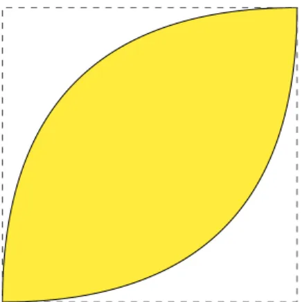
The computation is easy when d= 2. Thenv= (t,−s) withs, t≥0 and s+t= 1, say. Then4∩C(v≥0) is a triangle with vertices (0,0),(1,0),(s, t).
The integral in question is equal to the area of the triangle (which is t/2) times its centre of gravity (which equals (1 +s, t)/3). Using s= 1−t and suitable scaling we gett(v) = (2t−t2, t2). Withx, ycoordinates this is just x+y= 2√
y (for x≥y), a parabola arc. Thus the boundary ofT0 consists of two parabola arcs given by the equations x+y = 2√
y (for x ≤ y) and x+y = 2√
y (for x ≥ y), which is the same as the limit shape in R2 of convex lattice polygons, see Bárány [1] and Vershik [15].
Figure 1. The limiting zonoid in dimension 2.
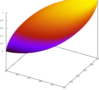
The same method works inR3. This time the previous triangle is replaced by the simplex with vertices (0,0,0),(1,0,0),(s, t,0),(u,0, v) withs, t, u, v≥ 0 and s+t = 1 u+v = 1. The integral in question is the volume of this simplex (tv/6) times its centre of gravity ((1 +u+s, t, v)/4). Usings= 1−t and u = 1−v again we get t(v) = (3tv−t2v−tv2, t2v, tv2) . Thus the equation of the boundary of T0 is x+y + z = 3√3
yz; this holds when x−2y+z≥0 andx+y−2z≥0, as one can check directly. T0 is centrally symmetric with respect to center (1/2,1/2,1/2). Its boundary is made up of six pieces that come in symmetric pairs. The piece in the region determined by inequalities x−2y+z≥0 and x+y−2z≥0 is given by the equation x+y+z= 3√3
yz. Other pieces are given by equationsx+y+z = 3√3 xz and x+y+z= 3√3
xy, and the reflections with respect to the center.
The same method works in higher dimensions. There 4 ∩C(v ≥ 0) is not a single simplex, one has to triangulate it into simplices, and on each simplex, the integral in question can be computed the same way as above. We have not carried out this computation. Yet one can show that a certain part of the boundary of T0 in Rd is described by the equation x1+. . .+xd=d(x2. . . xd)1/d.
0 0.2
0.4 0.6
0.8 1 0
0.2 0.4
0.6 0.8
1 0
0.2 0.4 0.6 0.8 1
Figure 2. The limiting zonoid in dimension 3.
The same limit shape comes up in another way as well. We are going to explain, rather informally, how this happens. We start with a simple proposition.
Proposition 3.2. Assume S ⊂ C is a closed set and RSxdx = a. Then VolS≤q(C,a) and equality holds iff S =Q(C,k).
Proof. It is clear thatRSxdx=a implies thatRSu·xdx=u·a. Note that R
Qu·xdx=u·a as well. Then Z
S\Q
u·xdx= Z
Q\S
u·xdx.
The value ofu·xis larger onS\Qthan onQ\S. This shows that VolS\Q is smaller than Vol(Q\S) unless both are equal to zero.
Assume that k ∈ Zd∩IntC and consider the cap Q(C, nk) when n is large. DefineVn=Zd∩Q(C, nk). It is known (and follows from an estimate similar to the one in Lemma A.2) that, as ngoes to infinity,
X
x∈Vn
x=nk(1 +o(1)).
Suppose now thatPx∈Sx=nkfor someS ⊂Zd∩C. Under these conditions Proposition 3.2 implies that |S| ≤ |Vn|(1 +o(1)).
This shows that the (asymptotically) largest setS⊂Zd∩CwithPx∈Sx= nk is Vn. The integral zonotope T(Vn) has its endpoint close to nk. The limiting zonoid T0(C,k) from Theorem 1.1 turns out to be the limit of the zonotopes n1T(Vn) as n→ ∞.
4. The probabilistic approach
Throughout this paper we work under the following condition:
(4.1) C∈ Cd and k∈IntC∩Zd are fixed.
In this section, we give a proof of Theorem 1.1 and Theorem 1.2 based on statistical mechanics techniques. Obviously, the statement of the theorem itself is already of probabilistic nature.
4.1. Description of the model. Let Ω be the set of all functions from Pd ∩C to Z+ with finite support. Recall from Section 2 the correspon- dence between lattice zonotopes, strict integer partitions, and multiplicity functions ω ∈ Ω. In particular, each function ω is associated to a unique zonotope T(ω), and conversely. Moreover, the endpoint ofT(ω) is
X(ω) = X
x∈Pd∩C
ω(x)x.
The probability distribution Qn on Ω, which is defined for all ω∈Ω by Qn(ω) = 1
p(C, nk)1{X(ω)=nk}
is exactly the uniform distribution on T(C, nk). The conclusion of Theo- rem 1.1 can be stated as convergence in probability for this distribution:
dist(n1T, T0)−−−→Qn
n→∞ 0.
We now define a new probability distribution Pn on Ω, which will turn out to behave roughly like Qn when n tends to +∞. It depends on two parameters u and βn fixed throughout the paper as follows:
(4.2) u=u(C, λk), βn= d+1
sζ(d+ 1) ζ(d)
1 n,
where u(C, λk) =λ−1u(C,k)∈C◦ is defined by Theorem 3.1, with λ >0 chosen such that
(d+ 1)!
Z
C(u≤1)
xdx=k.
The reason for these choices will become apparent in Proposition 4.1. The probability distribution Pnis then defined for all ω ∈Ω by
Pn(ω) = 1 Zn
e−βnu·X(ω), whereZn= X
ω∈Ω
e−βnu·X(ω).
This definition, which is directly inspired by statistical mechanics, is a special case of the Boltzmann distribution. It is a generalization of the model introduced by Sinai [13] for convex lattice polygonal lines. Here Zn is the so-calledpartition function of the model. The sum definingZnis easily seen to be convergent.
The crucial observation is the following: since Pn(ω) only depends on the value X(ω), we see that for allm∈Zd,
(4.3) Pn[X=m] = p(C,m)
Zn e−βnu·m.
In particular, the distribution induced on Ω by Pn conditional on the event {X=nk}is exactly Qn. For all events E⊂Ω,
Qn[E] = Pn[E |X=nk] = Pn[E∩ {X=nk}]
Pn[X=nk] .
Consequently, our strategy of proof for Theorem 1.1 is to establish first a strong limit shape result for the distribution Pn and then use this relation with E ={dist(n1T, T0) > ε} to get the result for Qn. This deduction will only be possible if we show that Pn[X=nk] is not too small.
In comparison with Qn, the distribution Pn has a much simpler proba- bilistic structure. It is a product distribution on Ω since, by definition of X,
e−βnu·X(ω)= Y
x∈Pd∩C
e−βnω(x)u·x.
Thus, the family of random variables (ω(x))x∈Pd∩C is independent under Pn. In addition, one can see that for all x ∈ Pd∩C, the integer-valued random variable ω(x) has geometric distribution with parameter e−βnu·x (failure probability), that is to say
(4.4) Pn[ω(x) =i] = (1−e−βnu·x)e−iβnu·x, i∈Z+.
These two facts lead to a remarkable factorization ofZnas convergent prod- uct which is similar to Euler’s formula,
Zn= Y
x∈Pd∩C
1 1−e−βnu·x.
Taking logarithms, we obtain finally a series expansion for logZn,
(4.5) logZn= X
x∈Pd∩C
X
r≥1
e−rβnu·x
r .
The same expression is used in [1] and [13].
4.2. Asymptotic behaviour after rescaling. In this section, we inves- tigate the asymptotic distribution of the random vector X. It turns out that, after a proper rescaling, it can described completely by the Laplace transform (also called a characteristic function in [8]) of the cone C, which is defined by
ΛC(v) = Z
C
e−v·xdx, v∈C◦.
When there is no risk of confusion with another cone, we write Λ = ΛC. Proposition 4.1. Let µn and Γn denote respectively the mean value and the covariance matrix of the random vector X under the distribution Pn. Then
(4.6) lim
n→+∞
1
nµn=−∇Λ(u) =k, and lim
n→+∞n−d+2d+1Γn=∇2Λ(u), where ∇Λ and∇2Λdenote respectively the gradient and the Hessian matrix.
Moreover, the distribution of X satisfies a central limit theorem in the sense that
Γ−1/2n (X−µn)−−−−−law→
n→+∞ N(0, Id).
Proof. We introduce a function Z :C◦ →R+ such that Zn=Z(βnu). It is defined for all v∈C◦ by
Z(v) = X
ω∈Ω
e−v·X(ω).
Let β = βn in the proof. We start with the statement about µn. It is a well known fact that in such an exponential model, the first moments of X are given by the logarithmic derivatives of the functionZ. In the case of the mean value, it results from the following simple computation:
µn= En[X] = X
ω∈Ω
e−βu·X(ω)
Z(βu) X(ω) =−∇Z(βu)
Z(βu) =−∇logZ(βu).
Now, a straightforward generalization of formula (4.5) to the function Z leads to a series expansion of ∇logZ, namely
−∇logZ(βu) =X
r≥1
X
x∈Pd∩C
e−rβu·xx.
For every index r less than 1/β, we approximate the summation onPd∩C with the corresponding d-dimensional integral by using Proposition A.1.
Since the terms withr >1/β contribute onlyO(1/β), we obtain after sum- mation
µn= 1 βd+1
ζ(d+ 1) ζ(d)
Z
C
e−u·xxdx+O 1
βd
in the limit β →0. The integral here is obviously−∇Λ(u). We need check that it is also equal to k. This is done by applying the fundamental theorem of calculus and the Fubini-Tonelli theorem:
Z
C
e−u·xxdx= Z
C
Z ∞ u·x
e−tdtxdx= Z ∞
0
e−t Z
C(u≤t)
xdxdt.
An homothetic change of variable yields therefore by homogeneity:
Z
C
e−u·xxdx= Z ∞
0
td+1e−tdt Z
C(u≤1)
xdx= (d+ 1)!
Z
C(u≤1)
xdx=k.
So the first part of the proposition is finally proven by replacing β with its expression as a function of n.
The proof of the asymptotic behaviour of the covariance matrix Γn is entirely similar except that we consider the second order derivatives of the logarithmic partition function. We omit the details.
We now turn to the central limit result. Recall that the random variables ω(x) are independent and eachω(x) follows the geometric distribution with parametere−βu·x. In particular, Γ−1/2n (X−µn) is the sum of the independent random variables (ω(x)−E[ω(x)]) Γ−1/2n x of mean value 0. We are going to check the classical Lyapunov condition on third moments, which implies the central limit theorem for independent, but not necessarily identically distributed, summands. We must show that
Ln= X
x∈Pd∩C
E
(ω(x)−E[ω(x)]) Γ−1/2n x3
goes to 0 as n tends to +∞. Elementary computations on the geometric distribution yield, for all x∈Pd∩C,
E[ω(x)] = e−βu·x
1−e−βu·x, and Eh|ω(x)−E[ω(x)]|3i≤ 3e−βu·x (1−e−βu·x)3. Letting kΓ−1/2n k denote the operator norm, we obtain therefore,
Ln≤3kΓ−1/2n k3 X
x∈Pd∩C
kxk3e−βu·x (1−e−βu·x)3.
From the first part of the proposition, we already know that kΓ−1/2n k is of order n−12(d+2)/(d+1). Moreover, Proposition A.1 shows that
X
x∈Pd∩C
kxk3e−βu·x
(1−e−βu·x)3 and nd+3d+1 Z
C
kxk3e−u·xdx
are of the same order of magnitude as n tends to +∞. Accordingly, Ln
is at most of order n−d/(2d+2), hence tends to 0 and we can indeed apply Lyapunov’s central limit theorem. The proof is complete.
Letting σn=n2d+2d+2, the central limit theorem of Proposition 4.1 can now be stated as
(4.7) X−nk
σn
−−−→law
n→∞ N(0,∇2Λ(u)).
The proof of the next proposition will use this fact.
Proposition 4.2 (Weak local limit estimate).
Pn[X=nk] =e−o(nd/(d+1))
Proof. We begin with the following simple remark: if m ∈ Zd∩C and n ∈ Zd∩C satisfyn−m∈C, then p(C,n) ≥p(C,m). This explains the introduction of the following set,
An={m∈Zd∩C |nk−m∈C andu·(nk−m)≤σn}.
As a consequence of (4.7), there exists c >0 such that Pn[X∈An]≥c for all nlarge enough. In addition, equation (4.3) and the remark above imply that
Pn[X∈An] = X
m∈An
p(C,m)e−βnu·m
= X
m∈An
p(C,m)
p(C, nk)eβnu·(nk−m)Pn[X=nk]
≤ |An|eβnσnPn[X=nk].
Sinceσn=n(d+2)/(2d+2), the factor|An|=O(σnd) grows only as a power ofn while eβnσn =eO(nd/(2d+2)). Since Pn[X∈An]≥c, the result is proven.
4.3. The number of generators ofT ∈ T(C, nk). Zonotopes inT(C, nk) have been identified with functions ω : Pd∩C → Z+ with finite support.
The generators of T ∈ T(C, nk) are those x ∈ Pd for which ω(x) > 0, we write G(T) for the set of generators of T. Using the method of the previous subsection we determine the expected numberµn of the number of generators of T ∈ T(C, nk), under the distribution Pn. By Proposition 4.2, it will also lead to an estimate under the uniform distribution QnonT(Cnk).
Lemma 4.3.
µn= E[|G(T)|] = 1
ζ(d)βndΛC(u)(1 +O(βn)).
Proof. Letβ =βnin the proof. Formula (4.4) implies that Pn[ω(x)>0] =e−βu·x.
A consequence of Proposition A.1 is that
X
x∈Zd∩C
e−βu·x− 1 ζ(d)
Z
C
e−βu·xdx
≤ cd
βd−1, for some constant cd>0 depending on the dimension. Here
Z
C
e−βu·xdx= 1 βd
Z
C
eu·xdx= 1
βdΛC(u), and so
µ= 1
ζ(d)βdΛC(u)(1 +O(β)).
As βn−d = Θnd/(d+1) follows from the definition of β, the order of magnitude of µis nd/(d+1).
We will need a similar result for the number of generators lying in a hyperplane H.
Lemma 4.4. AssumeH is a hyperplane inRd containing the origin. Then µH = E[|G(T)∩H|] =O(n(d−1)/(d+1)),
where the implicit constant in O(·) is independent of H.
Proof. Letβ =βnin the proof. Following the above argument, we have µH = E[|G(T)∩H|] = X
x∈Zd∩C∩H
e−βu·x. The one-sided estimate of Lemma A.4 gives now that
X
x∈Zd∩C∩H
e−βu·x≤ζ(d)−1 Z
C∩H
e−βu·xdx+ cd−1
βd−2.
Here Z
C∩H
e−βu·xdx= 1 βd−1
Z
C∩H
eu·xdx.
Thus indeed
µH ≤ 1 +o(1) ζ(d)βd−1
Z
C∩H
e−u·xdx=O(n(d−1)/(d+1)).
4.4. Limit shapes. In this section, we are going to show the existence of a limit shape for random zonotopes drawn under the uniform distribution on the set of all lattice zonotopes in the cone C with endpoint nk.
For every convex compact subset A of Rd, the support function of A is the continuous function hA:Rd→Rdefined by
hA(w) = sup{v·w, v∈A}, w∈Rd. Let T0 =T0(C,k) be the zonoid defined in Section 3.
Theorem 4.5. For all v∈Rd and for all ε >0,
n→+∞lim Qnh|h1
nT(v)−hT0(v)|> εi= 0.
Proof. Again, the proof of this theorem is based on the probabilistic model of Section 4. It depends on the fact that, conditional on the event X=nk, the distribution of a random zonotope under Pn is uniformly distributed on the set T(C, nk). In particular,
Qnh|h1
nT(v)−hT0(v)|> εi= Pnh|h1
nT(v)−hT0(v)|> ε|X=nki
≤
Pnh|h1
nT(v)−hT0(v)|> εi Pn[X=nk] .
Hence, we only need to prove that the right-hand side of this inequality goes to 0. It is natural to consider only v ∈Sd−1, the unit sphere of Rd. Using Proposition 4.2, we see that the theorem follows from the result of the next
proposition.
Proposition 4.6. For allε >0 there existsc >0 such that for allv∈Sd−1 and for all n large enough,
Pnh|h1
nT(v)−hT0(v)|> εi≤exp{−c nd/(d+1)}.
Proof. It is evident that for a zonotope T(ω) generated by the vectorsx ∈ Pd∩C with multiplicitiesω(x) the support function is
hT(v) = X
x∈Pd∩C
ω(x)x·v 1{x·v≥0} = X
x∈Pd∩C(v≥0)
ω(x)x·v.
In the proof of Proposition 4.1, we could replace C with the smaller cone C(v≥0) and we would obtain
1
n En[hT(v)] = ΛC(v≥0)(u)·v+O(n−1/(d+1)) =hT0(v) +o(1).
Since n1hT =h1
nT, this already shows that the limit shape appears in expec- tation.
We will now bound the probability for a large deviation from the mean using the so-called Chernoff method. Let us consider the exponential gen- erating function of hT(v)
E[eθhT(v)] = Y
x∈Pd∩C(v≥0)
1−e−βu·x
1−e−(βu−θv)·x = ZC(v≥0)(βu−θv) ZC(v≥0)(βu)
which is well defined for all θ small enough with respect to β. Consider now the centered random variable Y = h1
nT(v) −E[h1
nT(v)]. The cen- tral limit part of Proposition 4.1 applies to the cone C(v ≥ 0) with k0 =
−∇ΛC(v≥0)(u). Thus by second order Taylor approximation, we obtain for some constantc(u,v)>0 involving the Hessian matrix of ΛC(v≥0) atu,
log E[eθY]∼c(u,v)θ2
2n−d/(d+1)
as long as nθ goes to 0. But for allθ >0, the Markov inequality yields Pn[Y > ε] = Pn[θY ≥θε]≤e−θεE[eθY]
This bound is approximately optimized for θ = c(u,v)−1ε nd/(d+1) and it leads to
Pn[Y > ε]≤exp
−1
2c(u,v)−1ε2nd/(d+1)(1 +o(1))
A similar bound holds for Pn[−Y > ε], hence for Pn[|Y|> ε]. The conclusion
follows.
4.5. The number of zonotopes. This section is devoted to the proof of Theorem 1.2, which states that
logp(C, nk) nd+1d
−−−→n→∞ cdq(C,k), where cd= d+1
sζ(d+ 1)
ζ(d) (d+ 1)!
and where q(C,k) is defined in Section 3 as the minimal volume of a cap of the cone C having kas its center of gravity.
The starting point of the proof is the equation (4.3) established earlier which links the number logp(C,k) with the probability distribution Pn in the following way:
logp(C,k) = logZn+nβnu·k+ log Pn[X=nk].
The value ofβnwas given explicitly by (4.2) and it shows thatnβnis of order nd/(d+1). On the other hand, we know by Proposition 4.2 that log Pn[X = nk] is negligible compared to nd/(d+1).
It only remains to estimate the term logZn. This is done by using the series expansion (4.5) and applying Proposition A.1 from the appendix in the same lines as the first part of the proof of Proposition 4.1. This leads to
logZn= ζ(d+ 1) ζ(d)
1
βnd(Λ(u) +o(1)),
which is again of ordernd/(d+1). A simple computation based on the defini- tion of βn and of the constant cdyields therefore
logp(C, nk) nd+1d
−−−→n→∞
cd
d+1p
(d+ 1)!(Λ(u) +u·k).
The final step is to express Λ(u) +u·k in terms of q(C,k). Recall that u is defined by (4.2) and that we have shown in Proposition 4.1 that
k= (d+ 1)!
Z
C(u≤1)
xdx= Z
C
xe−u·xdx.
The computation of Λ(u) +u·kis thus simply a matter of integral calculus.
Using the fundamental theorem of calculus and the Fubini-Tonelli theorem, we obtain:
Λ(u) +u·k= Z
C
(1 +u·x)e−u·xdx
= Z
C
Z ∞ u·x
t e−tdt dx
= Z ∞
0
te−tVolC(u≤t)dt
= (d+ 1)! VolC(u≤1)
Finally, the definition (4.2) of u and the considerations of volumes in Sec- tion 3 show that
VolC(u≤1) =q(C,(d+1)!1 k) = 1
(d+ 1)!
d
d+1q(C,k).
The proof is complete.
Remark. Although we did not use it directly, it appears above that u is actually the unique minimizer of the quantity Λ(v) +v·kforv∈C◦. This fact can be used to prove Gigena’s Theorem 3.1.
5. Number of vertices of a random zonotope
In this section we determine the order of magnitude of the expected num- ber of faces of each dimension and towers of a random zonotope. A tower (or flag) of a zonotope T is a chain F0 ⊂F1 ⊂. . . ⊂Fd−1, where Fi is an i-dimensional face of T. We denote by fi(T) the number of i-dimensional faces and by F(T) the number of towers of T.
Theorem 5.1. There are constants c1, c2 not depending on n such that
n→+∞lim Qn
T ∈ T(C, nk)|c1< fi(T)
nd(d−1)/(d+1) < c2
= 1,
n→+∞lim Qn
T ∈ T(C, nk)|c1< F(T)
nd(d−1)/(d+1) < c2
= 1.
As Qn is the uniform distribution on T(C, nk) the above theorem says that, asn→ ∞, for the overwhelming majority of the zonotopes inT(C, nk) the face numbers fi(T) and F(T) are of order nd(d−1)/(d+1). It is shown in [4, 12] that for any integer lattice polytope P with volP >0,
F(P) =O(volP)(d−1)/(d+1) .
The same upper bound for eachfi(P) follows immediately. Combined with the previous result on the volume of a random zonotope, this establishes the upper bounds of Theorem 5.1. It only remains to show the lower bounds.
5.1. Generators of a random zonotope. Let Tε(C, nk) consist of all zonotopesT ∈ T(C, nk) such that
|G(T)| ≥(1−ε)ζ(d)−1ΛC(βu),
and the number of generators of T that are contained in any single hyper- plane is at mostεΛC(βu). Our goal in this section is to prove all except for a minute fraction of the zonotopes in T(C, nk) belong toTε(C, nk).
Proposition 5.2.
n→+∞lim Qn[Tε(C, nk)] = 1.
Proof. This is quite easy. We rely on the two lemmas in Subsection 4.3 and on the following rough form of the Chernoff bounds:
Proposition 5.3(Chernoff bounds). LetX1, . . . , Xnbe independent Bernoulli random variables, let X=X1+. . .+Xn, and let µ= E[X]. For any δ >0,
P[X ≥(1 +δ)µ]≤e−δ2µ/3, 0< δ <1, P[X ≥(1 +δ)µ]≤e−δµ/3, 1≤δ, P[X ≤(1−δ)µ]≤e−δ2µ/2, 0< δ <1.
By Lemma 4.3 µ = E[|G(T)|] is of order nd/(d+1), and so an application of the Chernoff bound gives, that for any 0< ε <1
Pn[|G(T)| ≤(1−ε)µ]≤e−ε2µ/2 = exp{−cnd/(d+1)} where c >0 is a constant independent ofn.
Next, we bound the probability that a hyperplaneH with 0∈H contains more than a constant fraction of the expected number of generators of a zonotope in T(C, nk). According to Lemma 4.4, µH = E[|G(T)∩H|] ≤ cn(d−1)/(d+1) with c not depending on H and n. Applying the Chernoff bound with γ >1, we have
Pn[|G(T)∩H| ≥(1 +γ)µH]≤e−γµH/3. In particular,
Pn[|G(T)∩H| ≥εΛC(βu)]≤exp{−cnd/(d+1)} for some c >0 depending onε.
Note finally that the total number of hyperplanes (containing the ori- gin) spanned by the generators of a zonotope withO(nd/(d+1)) generators is bounded by O(nd(d−1)/(d+1)). Since this is polynomial in n, a union bound
proves Proposition 5.2.
5.2. Faces of a random zonotope. In this section, we show that the zono- topes inTε(C, nk) have at least the number ofi-dimensional faces prescribed by Theorem 5.1; the same lower bound for towers is an immediate corollary.
We rely on the following well-known duality between zonotopes and hy- perplane arrangements. An arrangement of hyperplanes is a finite collection of affine hyperplanes, together with their subdivision of Rd into relatively open cells. A central hyperplane arrangement is the decomposition of Rd induced by linear hyperplanes. For a d-dimensional zonotope T with gen- erators {v1, . . . ,vm}, let Ac(T) be the central arrangement of hyperplanes with this set of normal vectors. The number of k-dimensional cells ofAc(T) is equal to the number of d−k faces of T (see, e.g., [6, Prop. 2.2.2]). Let A(T) be the (d−1)-dimensional arrangement of affine hyperplanes obtained as the intersection ofAc(T) with a generic hyperplane. Clearly, the number
of (k−1)-dimensional cells of A(T) is a lower bound on the number of k- dimensional cells ofA(T) fork∈[1, d]. We note that twice this lower bound is an upper bound on the number in question as the cells of Ac(T) come in pairs C,−C exceptC ={0}.
Proposition 5.4. There is a constant c independent of n such that for all ε ∈ (0, c) and T ∈ Tε(C, nk), we have fi(T) = Ω(nd(d−1)/(d+1)) for each 0≤i≤d−1.
Proof. If a single line {λv | λ∈ R} is incident to k hyperplanes of Ac(T), then the vector vis orthogonal tokgenerators of T. Since at most (ε/(1− ε))|G(T)| of the generators of T lie in the hyperplane v⊥ (for any v), the same bound applies to the maximum number of hyperplanes of A(T) that are incident to any single point. Hence, we can apply the following theorem of Beck [5] to bound the number of vertices of A(T).
Lemma 5.5. There is a constant c depending on dimension such that the following holds. Let A be an arrangement of m hyperplanes in Rd−1. Then either
(1) a single vertex of A is incident tocm hyperplanes of A, or (2) the total number of vertices in A isΩ(md−1).
Since A(T) is an arrangement of nd/(d+1) hyperplanes, this implies that, for εsufficiently small, the number of vertices ofA(T) is Ω(nd(d−1)/(d+1)).
Designate a generic direction winRd−1 to be “up”. Clearly, each (d−1)- dimensional region ofA(T) that is bounded from below has a bottom vertex.
We claim that each vertex ofA(T) is the bottom vertex of at least one region.
Let p be an arbitrary vertex of A(T). At least d−1 hyperplanes having linearly independent normals are incident to p. Let S be an arbitrary set of d−1 such hyperplanes. At least one (d−1) dimensional region R of A(T) is above each of these hyperplanes with respect to w, and p is the bottom vertex of each such region. In addition, p is the bottom vertex of each j-dimensional region that is contained in a hyperplane of S and that bounds R, for 1≤j ≤ d−2. Hence, the number of j-dimensional regions that are bounded below in A(T) is at least the number of vertices ofA(T), which is Ω(nd(d−1)/(d+1)).
Since the j-dimensional regions ofA(T) are in bijection with the (d−j)- dimensional faces of T, this completes the proof of the proposition.
5.3. A short digression. This proof method has an interesting conse- quence about hyperplane (or rather subspace) arrangements that seems to be new. Recall first that ifAis a central arrangement ofm general position hyperplanes in Rd, then fi(A) is known precisely for all i:
fi(A) =
k
X
k=d−i
k d−i
! m k
!
see for instance Buck [7] and Zaslavski [16]. Moreover, this function is an upper bound on the number of i-dimensional cells of every central arrange- ment of m linear hyperplanes in Rd. Define Acr as the collection of all d−1-dimensional subspaces of the form z⊥ where z ∈ Zd has Euclidean
length at most r. We could not find the following result anywhere in the literature or in folklore.
Theorem 5.6. The number of i-dimensional cells for all i= 1, . . . , d and the number of towers of Ar isΘ(rd(d−1)).
Proof. It follows from the result of Beck [5] cited above that the number of one-dimensional cells ofAcr is Θ(rd(d−1)). The same estimate is also implied by Theorem 3 of [3].
Let Ar be the (d−1)-dimensional arrangement of affine hyperplanes ob- tained as the intersection of Acr with a general position hyperplane H the same way as above. The previous proof applies word by word.
6. Integral zonotopes in convex bodies
As it is mentioned in the introduction, for d = 2 Theorem 1.1 follows from the results of Bárány [2]. In fact, more is true. We set up the question more generally. Assume K ⊂ Rd a convex body (i.e., convex compact set with non-empty interior) and write P(K, n) for the collection of all convex
1
nZd-lattice polytopes contained inK,P(K, n) is a finite set. It is proved in [2] that, whend= 2, the polygons inP(K, n) have a limit shape asn→ ∞:
Theorem 6.1. For every convex bodyK in R2 there is a convex bodyK0 ⊂ K such that, as n → ∞, the overwhelming majority of the polygons in P(K, n) are very close toK0. More precisely for every ε >0
n→∞lim
card{P ∈ P(K, n)|dist(P, K0)> ε}
cardP(K, n) = 0.
The distinguishing property of K0 is that its affine perimeter (for the definition see [2]) is maximal among all convex subsets of K. It is also shown there that such a K0 is unique. The analogous question in higher dimension is wide open. Even the case when K is the cube [−1,1]3 is not known.
Question 1. Assume K ⊂ Rd is a convex body and d > 2. Is there a limit shape to the convex polytopes in P(K, n)?
Define, similarly, F(K, n) as the collection of all convex n1Zd-lattice zono- topes contained in K,F(K, n) is again a finite set.
Question 2. Assume K ⊂ Rd is a convex body and d ≥ 2. Is there a limit shape to the convex zonotopes inF(K, n)?
We can answer this question when d= 2. Informally stating, for every convex body K in the plane there is a zonoid K0 contained in K such that, as n → ∞, the overwhelming majority of the polygons in F(K, n) are very close to K0. The proof follows the method of [2] so we only give a sketch. Note that in the plane a zonoid is always a centrally symmetric convex body and vice versa. The first thing to show is that K contains a centrally symmetric convex body that maximizes the affine perimeter among all centrally symmetric convex subsets ofK. This follows from the fact that the affine perimeter is upper semi-continuous. The next step is to prove that the maximizer is unique. Here one uses the fact that, for all t∈[0,1],