Állapotbecslés és állapotvisszacsatolás kvázi-polinomiális és kvantummechanikai rendszerekre

State estimation and state feedback control in quasi-polynomial and

quantum mechanical systems

PhD thesis

Written by: Attila Magyar Supervisor: Dr. Katalin Hangos

University of Pannonia

Information Science Ph.D. School

MTA SzTAKI

Systems and Control Laboratory

2007

State estimation and state feedback control in quasi-polynomial and quantum mechanical

systems

Ertekez´es doktori (PhD) fokozat elnyer´ese ´erdek´eben´

´Irta:

Magyar Attila

K´esz¨ult a Pannon Egyetem Informatikai Tudom´anyok Doktori Iskol´aja keret´eben T´emavezet˝o: Dr. Hangos Katalin

Elfogad´asra javaslom (igen / nem)

(al´a´ır´as) A jel¨olt a doktori szigorlaton ...%-ot ´ert el

Veszpr´em ...

a Szigorlati Bizotts´ag eln¨oke Az ´ertekez´est b´ır´al´ok´ent elfogad´asra javaslom:

B´ır´al´o neve: ... (igen / nem)

(al´a´ır´as)

B´ır´al´o neve: ... (igen / nem)

(al´a´ır´as)

A jel¨olt az ´ertekez´es nyilv´anos vit´aj´an ...%-ot ´ert el

Veszpr´em, ...

a B´ır´al´o Bizotts´ag eln¨oke

A doktori (PhD) oklev´el min˝os´ıt´ese ...

...

Az EDT eln¨oke

Tartalmi kivonat

Allapotbecsl´ ´ es ´ es ´ allapotvisszacsatol´ as kv´ azi- polinomi´ alis ´ es kvantummechanikai rendszerekre

A rendszer- ´es ir´any´ıt´aselm´elet ´allapott´er reprezent´aci´on alapul´o m´odszereit manap- s´ag olyan ter¨uleteken haszn´alj´ak, mint a robusztus, LPV, ´es LQ ir´any´ıt´as. Ezek az eszk¨oz¨ok olyan nehezen kezelhet˝o rendszerekre is alkalmazhat´oak, mint a folyamat- rendszerek, nukle´aris rendszerek, stb. Mindazon´altal, sz´eles m˝uk¨od´esi tartom´annyal rendelkez˝o er˝osen nemline´aris rendszerekre, mint a biomechanikai, biok´emiai, vagy kvantum rendszerek, jelenleg sincsenek j´ol alkalmazhat´o technik´ak.

A szerz˝o a disszert´aci´oban k´et - a fizika k¨ul¨onb¨oz˝o ter¨uleteir˝ol sz´armaz´o rendszer- oszt´alyon alkalmazta a modern ir´any´ıt´aselm´elet eszk¨ozeit. Kihaszn´alva a speci´alis rendszeroszt´alyok ny´ujtotta lehet˝os´egeket, siker¨ult gyakorlatilag megval´os´ıthat´o m´od- szereket adni olyan probl´em´akra, amelyek az ´altal´anos esetben neh´eznek, illetve sz´am´ıt´asig´enyesnek bizonyultak.

A folyamatrendszerek glob´alis stabilit´asvizsg´alat´at nemline´aris jelleg¨uk teszi ne- h´ez feladatt´a. Olyan speci´alis nemline´aris rendszermodell oszt´alyok alkalmaz´asa, melyek el´eg ´altal´anosak a folyamatrendszerek dinamikus viselked´es´enek le´ır´as´ara, megk¨onny´ıten´e ezen rendszerek ir´any´ıt´as´at. A szerz˝o a disszert´aci´oban az ´ugyneve- zett kv´azipolinomi´alis (QP) rendszeroszt´alyt alkalmazza a fenti c´elra. Kihaszn´alva, hogy QP rendszerekre a Ljapunov f¨uggv´eny alakja ismert, leegyszer˝us¨odik az ´altal´a- nos folyamatrendszerek glob´alis stabilit´asvizsg´alata. A kv´azipolinomi´alis rendszer- oszt´aly seg´ıts´eg´evel olyan szab´alyoz´otervez´esi feladatot is fel´ır, amely biztos´ıtja a z´art rendszer glob´alis stabilit´as´at egy adott Ljapunov f¨uggv´eny csal´adra n´ezve.

Mindezid´aig csup´an n´eh´any szerz˝o pr´ob´alta meg a kvantummechanikai rendsze- reket rendszerelm´eleti oldalr´ol megk¨ozel´ıteni. A disszert´aci´oban kit˝uz¨ott probl´ema kvantuminform´aci´o kiolvas´as´aval kapcsolatos. Kvantummechanik´aban a m´er´es va- l´osz´ın˝us´egi jelleg˝u m˝uvelet, ami a teljes rendszert sztochasztikuss´a teszi, ez´ert meg- b´ızhat´o ´allapotbecsl´esi m´odszerekre van sz¨uks´eg. Az egyik ´ut a bayesi m´odszertan alkalmaz´asa, amely egy teljes val´osz´ın˝us´egi modellt haszn´al, ´es az ez alapj´an sz´amolt becsl˝o sok statisztikai inform´aci´oval szolg´al a k´erd´eses ´allapotr´ol. A m´asik ir´anyt egy egyszer˝u pontbecsl˝o kifejleszt´ese jelenti, amely a kvantumrendszerek egy sz´elesebb oszt´aly´ara alkalmazhat´o, tov´abb´a a sz´am´ıt´asig´enye nem t´ul nagy.

Abstract

State estimation and state feedback control in quasi- polynomial and quantum mechanical systems

The goal of this dissertation is to apply system and control theory to two system classes originating from different fields of physics: process systems and quantum mechanical systems.

Using the quasi-polynomial system representation it is possible to describe the dynamic behavior of general nonlinear process systems. It is shown in the work, that global stability analysis for such systems can be performed algorithmically, moreover, a globally stabilizing state feedback design method is given.

Only a few authors tried to apply control theory in quantum mechanical fields.

The aimed problem of the second part of the dissertation is quantum state esti- mation, where the state of a quantum system is to be determined from quantum measurement. The problem is solved in two different ways.

Zusammenfassung

Zustandsch¨ atzung und R¨ uckkoppelung f¨ ur quasi- polynomischen und quantenmechanischen Systemen

Das Prim¨arziel dieser Dissertation ist die Anwendung der Ergebnisse der System- und Regelungstheorie auf zwei verschiedene Systemsklassen der Physik: Prozess- Systeme und quantenmechanische Systeme.

Mit der Hilfe der quasi-polinomischen Systemklassen kann man die dynamischen Verhaltensweise des allgemeinen Prozesssysteme beschreiben. Der Autor will in der Dissertation zeigen, dass die globale Stabilit¨atspr¨ufung des quasipolinomischen Systemen algorithmisch ausgef¨uhrt werden kann. Ausserdem demonstriert er eine global stabilisierende R¨uckkoppelungs-Planungsmethode.

Bisher haben nur Wenige versucht die Systemtheorie im quantummachanischen Bereich anzuwenden. In dem zweiten Teil der Dissertation sind L¨osungsm¨oglichkeiten des Problems der Zustandsch¨atzung vom quantummechanischen Messungen gezeigt.

Zur Erzielung dieser L¨osung muss der Systemzustand vom Quantenmessungen aus- wertet werden. Der Autor zeigt zwei Methoden f¨ur die L¨osung der Aufgabe.

Acknowledgement

First of all I would like to express my gratitude to Dr. Katalin Hangos, my super- visor, for her help. She gave me a lot of advice and guidance in my research, helped me with my studies, and gave me inspiration for my future work.

I would also like to thank Dr. J´ozsef Bokor, Head of Systems and Control Laboratory, Computer and Automation Research Institute, for making my research possible, I am grateful to Dr. G´abor Szederk´enyi, the coauthor of most of my papers for his help and advices. I would like to thank Dr. D´enes Petz for his help in the quantum mechanical part of my work. I am also grateful to my research fellows, D´avid Csercsik, Csaba Fazekas, Dr. Erzs´ebet N´emeth, L´aszl´o Ruppert and Zsuzsanna Weinhandl for their cooperation. I am grateful for all the help I received from every member of our Laboratory.

Finally, I am also grateful to my family for the strong support they gave me in the past 28 years.

Contents

1 Introduction 10

1.1 Background and motivation . . . 10

1.2 System- and control theory. . . 11

1.3 Problem statement and aims . . . 13

1.4 Thesis structure . . . 14

1.5 General notations . . . 15

I QP systems 17

2.1.1 QP models. . . 19

2.1.2 Lotka-Volterra models . . . 19

2.1.3 Input-affine QP system models . . . 20

2.2 Embedding process systems into QP and LV forms . . . 21

2.2.1 QP models of process systems . . . 22

2.2.2 A simple fermentation example . . . 22

2.3 Earlier work on the representation of QP systems . . . 25

3 Stability analysis of quasi-polynomial systems 26 3.1 Global stability analysis using linear matrix inequalities . . . 26

3.1.1 Global stability analysis . . . 26

3.1.2 Zero dynamics analysis . . . 27

3.1.3 Zero dynamics of the simple fermentation process . . . 28

3.2 Time-reparametrization. . . 29

3.2.1 The time-reparametrization transformation . . . 29

3.2.2 Properties of the time-reparametrization transformation . . . 30

3.2.3 The time-reparametrization problem as a BMI . . . 31

3.2.4 Examples . . . 33

3.3 Summary . . . 34

4 Stabilizing control of quasi-polynomial systems 35 4.1 The controller design problem . . . 35

4.2 Numerical solution of the controller design problem . . . 36

4.2.1 Numerical solution based on bilinear matrix inequalities . . . 36

4.2.2 An iterative LMI approach to controller design problem . . . . 37

4.3 Equilibrium points . . . 39

4.3.1 Fully actuated case . . . 40

4.3.2 Partially actuated case . . . 40

4.3.3 Rank deficient (embedded) systems . . . 40

4.4 Feedback structure selection . . . 41

4.4.1 Fully actuated case . . . 41

4.4.2 Partially actuated case . . . 42

4.4.3 Degenerated case . . . 42

4.5 Examples . . . 42

4.5.1 Partially actuated process system example in QP-form . . . . 43

4.5.2 Fully actuated process system example in QP-form . . . 44

4.6 Summary . . . 45

II Quantum systems 47

5.1.1 Quantum dynamics . . . 49

5.1.2 State representation: the density matrix . . . 50

5.1.3 Finite quantum systems . . . 51

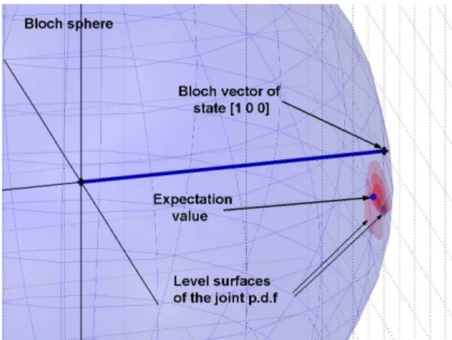
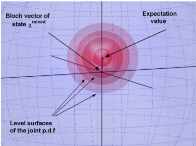
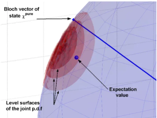
5.1.4 Bloch vector . . . 51

5.1.5 Distances between quantum states . . . 53

5.2 Quantum measurement and state estimation . . . 54

5.2.1 von Neumann measurement . . . 54

5.2.2 Positive operator valued measurement . . . 55

5.2.3 The quantum state estimation problem . . . 56

5.3 Earlier work on quantum state estimation . . . 57

6 Bayesian state estimation of a quantum bit 58 6.1 Componentwise estimation of the Bloch vector . . . 58

6.1.1 Bayesian estimate . . . 58

6.1.2 Point estimate. . . 60

6.2 Estimation of the Bloch vector . . . 61

6.2.1 Unconstrained Bayesian estimation . . . 61

6.2.2 Constrained Bayesian estimation . . . 61

6.3 Comparison based on computer simulation results . . . 62

6.3.1 A simulation software for quantum systems. . . 62

6.3.2 The effect of the number of measurements . . . 62

6.3.3 The effect of the length of Bloch vector . . . 64

6.4 Summary . . . 66

7 Point estimation of N-level quantum systems 68 7.1 The unconstrained estimation scheme . . . 68

7.1.1 Measurement strategy . . . 68

7.1.2 State estimator for N-level quantum systems . . . 69

7.1.3 Properties of the estimate . . . 70

7.2 The constrained estimation scheme . . . 73

7.2.1 The constrained estimator and its properties . . . 73

7.2.2 Computing the constrained estimate . . . 74

7.3 Comparison with other state estimation methods . . . 77

7.3.1 The modified unconstrained estimator . . . 79

7.3.2 Standard qubit tomography . . . 79

7.3.3 Minimal qubit tomography . . . 80

7.4 Summary . . . 81

8 Conclusions 82 8.1 Stability analysis and state estimation for state feedback . . . 82

8.2 New results . . . 83

8.3 Future work and applicability areas . . . 85

8.4 Own papers . . . 86

A Appendix 88 A.1 Basics of system and control theory . . . 88

A.1.1 System classes, basic system properties . . . 89

A.1.2 Controller design . . . 91

A.1.3 State estimation. . . 94

A.1.4 System parameter estimation . . . 95

A.2 Bloch vector space in the N-level case. . . 97

A.3 Examples of QP feedback design . . . 98

A.3.1 Example with a rank deficient M matrix . . . 98

A.3.2 Feedback design for a simple fermentation process . . . 100

A.4 Applied mathematical tools . . . 101

A.4.1 Linear and bilinear matrix inequalities . . . 101

A.4.2 Tensor product and its properties . . . 102

A.5 Tables . . . 103

A.6 Spinsim function reference . . . 104

Chapter 1 Introduction

Discovering the world is interesting, useful, delightful, terrifying or edifying;

discovering ourselves is the greatest journey, the most terrifying discovery and the most edifying of encounters.

/S´andor M´arai/

Analysis and control of general nonlinear and stochastic systems is a difficult area with many computationally hard problems. However, in special cases by using special system classes which exploit the physical characteristics of the examined system, feasible results can be achieved.

The present work connects two topics with different special system class and slightly different focus, that are originated from different fields of physics. However, they are connected through system- and control theory, and they represent two special, yet practically important nonlinear and stochastic system classes.

One of them is the class of lumped process systems with smooth nonlinearities that can be embedded into the class of quasi-polynomial systems. The other one is the class of finite quantum systems.

1.1 Background and motivation

Process systems appearing in practice [23] are difficult to handle since there are no universal methods which give a complete framework for their dynamical analysis, and synthesis [44]. That’s why it would be of great importance to develop methods which are general enough to handle a wide range of process systems, or to find a representation that’s suitable for describing almost all process systems. At the same time, process systems form a relatively simple nonlinear system class with smooth nonlinearities that are relatives of systems with polynomial nonlinearities. This is, why the quasi-polynomial system class has been selected as a case study for a class of ”easy” nonlinear systems.

On the other hand, one of the biggest challenge of present days is the built of a quantum computer which would make some special problems easier to solve (e.g.

prime factorization). These problems are tackled by quantum computation [1] and

quantum cryptography [5]. While classical computers manipulate classical informa- tion represented by systems obeying classical physics, quantum computers would modify, write, read quantum information which can be represented by quantum me- chanical systems. It means, that in order to be able to read quantum information we must be able to guess the actual properties of a quantum mechanical system from measurements performed on it [24].

From the system theoretical point of view, even the simplest quantum systems are unusual stochastic systems, where the stochastic nature is caused by the mea- surements that act as a disturbance to the system. This property causes that quan- tum systems represent a real challenge for everyone who attempts to solve even the simplest control-related problem for them.

Modern control methods for nonlinear and/or stochastic systems rely on the concept of state and apply state-space models. Therefore, state estimation and state feedback controller design are key problems in system and control theory.

1.2 System- and control theory

The general notion of system allows us to treat physical objects originating from various fields of life: automotive systems, chemical processes, nuclear powerplants, etc. System- and control theory (see Appendix A.1 for introduction of some basic notions, [2], or [9] for a deeper insight) allows us to examine and modify systems with mathematical tools.

Nonlinear systems

A wide class of dynamical systems can be represented by the following state space model [64]:

˙

x(t) =f(x(t)) + Xp

i=1

gi(x(t))ui(t) (1)

y(t) = h(x(t)) x(t₀) =x⁰,

where x(t)∈Rⁿ, u(t) = (u1(t), u2(t), . . . , up(t))^T ∈R^p and y(t)∈R^q, f :Rⁿ→Rⁿ, gi :Rⁿ →Rⁿ, i= 1, . . . , p, h:Rⁿ→R^q

are nonlinear functions. What makes (1) attractive is the fact that although the system is nonlinear in the states, it is linear in its inputs.

Dynamical analysis of nonlinear systems needs advanced mathematical tools [64], [29]. Global stability analysis of nonlinear systems calls for the searching of a suitable Lyapunov function V with the following properties:

• scalar valued function: V :Rⁿ →R⁺

• positive: V(x(t))>0

• decreasing in time: _dt^dV(x(t))<0

Although the form of the Lyapunov function is not known for a general nonlinear system (1), for some special system class (see Appendix A.1.1) it is possible to achieve results.

State feedback control

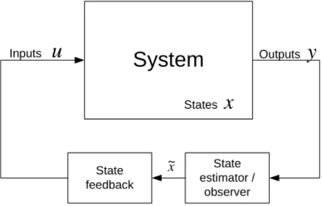
Applying control to the system makes it possible to modify its dynamical properties, and behavior. In most cases the control aim is reached by using feedback, i.e. the output signal is fed back to the input through a controller (see figure 1). In most cases, the structure of the controller is a state feedback, which means, that the control input is determined as a function of the states:

u(t) = k(x(t)), k:Rⁿ→R^p. (2) This implies a problem in the general case, since it is only possible to measure the outputs of the system. It explains the additional unit (the state estimator/observer) before the controller that computes the state signal from the output, as it can be seen in figure1.

System

State estimator /

observer State

feedback

Inputs

u

y

States

x

~x

Figure 1: State feedback control

State estimation

It was mentioned above, that most control techniques apply state feedback. This calls for a method that determines the actual state x of the system using the sup- posed system model and measured input-output data corrupted by some noise ac- cording to measurement devices. Such a method is called state estimation.

The state estimator is a mapping from the set D of possible measurement data to the state space:

ˆ

x=l(u,y),˜ l:D→Rⁿ, (3)

where ˆxdenotes the estimate of the statex, ˜ystands for the measured (and possibly noisy) output. A well known, and widely used tool for state estimation is the Kalman-filter [32].

Of course, a good estimate ˆx should meet some requirements. The first one is unbiasedness which means, that the expected value of the estimate ˆx equals to the real state x. Moreover, a consistent estimate is needed, i.e. an estimate that converges to the real state as the number of measurements increases.

System parameter estimation

Most of the controller design and state estimation methods need the dynamical model of the system, since the parameters of the controller and/or the state esti- mator/observer are computed from the system parameters. Estimating the model parameters [52], [54] is also a basis of system diagnostics since different parameter values may refer to certain faults of the plant.

The two fundamental methods of parameter estimation are the least squares estimation and the bayesian parameter estimation, they are summarized in the Ap- pendix A.1.4. Whilst the least squares (LS) estimation is based on minimizing the norm of the model error with a given parameter set, bayesian method uses a stochas- tic model of the system in the form of a conditional probability density function and gives more statistical information about the model parameters.

1.3 Problem statement and aims

The present thesis treats two different system classes originating from fields that are far away from each other. Tools of modern system and control theory are applied on them in such a way that their specialities are utilized to obtain practically feasible methods for problems that are computationally hard in the general case.

The nonlinear nature of general process systems makes their global stability analysis hard, however, in case of industrial process systems, like fermentation it is crucial to be able to prove the stability of a system to be implemented. Using nonlinear system model classes (more special than (1)) that is still general enough to describe the dynamics of them it might be easier to handle them.

In this work the so-called quasi-polynomial (QP) system class will be used for this purpose. QP systems has a very advantageous property, namely, the structure of their Lyapunov function is known. Using this fact will facilitate the global stability analysis of general process systems since it is only necessary to find suitable param- eters of a Lyapunov function of a given form in order to prove global asymptotic stability.

As a next step, the QP system class will be used for synthesizing controllers which ensure the global stability of the closed loop system with respect to the given Lyapunov function family. Using the fact, that with a suitable feedback the closed loop system still belongs to the class of QP systems, the same type of Lyapunov function can be used.

Note, that the state variables of process systems are typically concentrations, temperatures which are measurable quantities so the feedback control of them does not require state observers or estimators.

So far, only a few people (e.g. [38]) has tried to handle quantum mechanical systems on the control theoretical basis. The aimed subproblem of reading quantum information asks for the design of state observers/estimators. As it will be shown later in chapter 5 the measurement of a quantum system has probabilistic nature and turns the whole system to be stochastic (see (134) in Appendix A.1.1), reliable state estimation methods must be developed.

One way is to apply the Bayesian methodology (see AppendixA.1.4 for the basic

notations of the Bayesian parameter estimation problem) to use a full probabilistic model and give a state estimate that holds a lot of information about the state to be estimated.

The other direction to quantum state estimation is to develop a simple estimator which is applicable for a wide range of quantum systems and moreover it is easy to compute.

1.4 Thesis structure

This work is structured as follows. Present chapter clarifies the notations used throughout the work, and a short overview on system- and control theory is also presented here.

The results presented in this thesis are structured in two main parts. Part I is dedicated to quasi-polynomial model based dynamical analysis and control of process systems. Within this, chapter 2 gives an introduction to quasi-polynomial systems and their connection to nonlinear process systems. Chapter 3 links the global sta- bility analysis of quasi-polynomial systems to linear matrix inequalities. A bigger chance on proving global stability can be reached by the time-reparametrization transformation, which is also presented here. Chapter4 uses the results of the pre- vious chapter and deals with the design of a state feedback controller that globally stabilizes the system with respect to an entropy-like Lyapunov function.

The fundamental notions of quantum mechanics together with the proposed results pertaining to the state estimation of quantum systems are presented in part II. Within this, the basics of quantum mechanics used in the later chapters are summarized in chapter5. The next two chapters concentrate on the state estimation of quantum mechanical systems. Chapter 6 applies Bayesian methodology to the determination of states of single quantum bits. A more general class of quantum systems is treated in chapter 7by a simple but effective estimation procedure.

At the end of each chapter containing new results, a summary is presented. The own results are written in italic typeface. The corresponding publications are cited also in the title of each section.

Finally, chapter 8 summarizes all results, and the four suggested thesis points are also presented here together with my own papers. The future plans are also mentioned in chapter 8.

In the Appendix, one can find a brief summary of system- and control theory (Appendix A.1). Appendix A.2 the structure of N-level quantum systems’ Bloch vector space is detailed. Afterwards some examples connected to quasi-polynomial feedback design are given (AppendixA.3). In AppendixA.4, linear matrix inequal- ities, bilinear matrix inequalities are discussed together with the basic properties of the tensor product. The function reference of the quantum system simulator called Spinsim can be found in Appendix A.6.

1.5 General notations

The notations and abbreviations used throughout the work are summarized in this section. Since we are treating two fields in a common system theoretical framework, it is important to use a strict notation which makes it easier to find the connections between the two parts. The most important notations are listed below.

Notation - Meaning

x∈X - x is an element of set X x /∈X - x is not an element of setX X ⊂Y - X is a subset of Y

∅ - empty set

∪ - union

∩ - intersection

R - set of real numbers C - set of complex numbers Rⁿ - n dimensional real space

A - matrix

A^T - transpose of matrix A

A^∗ - conjugate transpose of matrix A A_i,j - (i, j)-th entry of matrix A

Ak - k-th element in a series of matricesA1, A2, . . . I - unit matrix of appropriate size I = diag(1, . . . ,1) E_ij - square matrix of appropriate size whose (i, j)-th

entry is 1, all the others are 0 TrA - trace of matrix A

detA - determinant of matrix A

A⊗B - tensor product of matrices A and B A◦B - Hadamard product of matrices A and B,

i.e. (A◦B)_i,j =A_i,jB_i,j c - scalar, or vector

ci - i-th element of vector c c^T - transpose of vector c

H - Hilbert space

|xi - vector from a Hilbert space, a ket state hx| - a bra state according to the ket |xi

S - system operator

x(t), or x - state of a given system,

or a Bloch vector of a quantum mechanical system

χ - density matrix

Notation - Meaning

Prob(ω) - probability of event ω

E ξ - expectation value of random variable ξ u(t), or u - input of a given system

y(t), or y - output of a given system

˙

x= ^dx_dt - time derivative of x

∂f(x)

∂xi - i-th partial derivative off(x) p(.) - probability density function

D^k - measurement data obtained fromk measurements

The abbreviations used in the sequel are the followings.

Abbreviation - Meaning

QP - quasi-polynomial

LV - Lotka-Volterra

GLV - generalized Lotka-Volterra

LS - least squares

RHS - right hand side

LMI - linear matrix inequality

ILMI - iterative LMI

BMI - bilinear matrix inequality LTI - linear time invariant

CSTR - continuously stirred tank reactor POVM - positive operator valued measurement p.d.f. - probability density function

iff - if and only if

s.t - such that

Throughout the thesis, my own papers are cited in the form [Oi], while other publications are cited as [j].

Part I

QP systems

Process systems are highly nonlinear systems due to some special features taking place in them [23]. Quasi-polynomial and Lotka-Volterra models have proved to be one of the candidates for generally applicable canonical forms of nonlinear process system models since the majority of smooth nonlinear systems occurring in practice can be transformed into these forms.

The aim of the first part is to utilize the quasi-polynomial and Lotka-Volterra representation to stabilizing control of process systems. Before formulating the feedback design problem the global stability analysis will be solved.

Chapter 2

Basic notions on quasi-polynomial systems

Present chapter gives a theoretical summary and a literature overview of part I.

Quasi-polynomial systems are introduced in section 2.1. Section 2.2 deals with the conditions and the algorithm of embedding general nonlinear process systems into quasi-polynomial form. At the end of the chapter a brief review of earlier works connected to the representation and stability analysis of quasi-polynomial systems is given (section 2.3).

2.1 Quasi-polynomial and Lotka-Volterra systems

The elementary notions in the field of quasi-polynomial (QP) and Lotka-Volterra (LV) systems are introduced in this chapter. In order to emphasize the similarity of QP and LV systems, QP systems are also called generalized Lotka-Volterra (GLV) systems.

2.1.1 QP models

Quasi-polynomial models are systems of ODEs of the following form

˙

xi =xi λi+ Xm

j=1

Ai,j

Yn

k=1

x^B_k^j,k

!

, i= 1, . . . , n. (4) where x ∈ int(Rⁿ

+), A ∈ R^n×m, B ∈ R^m×n, λi ∈ R, i = 1, . . . , n. Furthermore, λ = [λ1 . . . λn]^T. The above model belongs to the class of nonlinear systems (131), see Appendix A.1.1. Let us denote the equilibrium point of interest of (4) as x^∗ = [x^∗₁ x^∗₂ . . . x^∗_n]^T. Without the loss of generality we can assume that Rank(B) =n and m≥n (see [28]).

2.1.2 Lotka-Volterra models

The above family of models is split into classes of equivalence [27] according to the values of the products M =B ·A and N =B ·λ. The Lotka-Volterra form known

from the field of population biology [42], [65], gives the representative elements of these classes of equivalence. If rank(B) = n, then the set of ODEs in (4) can be embedded into the following m-dimensional set of equations, the so called Lotka- Volterra model:

˙

zj =zj Nj+ Xm

i=1

Mj,izi

!

, j = 1, . . . , m (5)

where

M =B ·A, N =B·λ, and eachzj represents a so called quasi-monomial:

zj = Yn

k=1

x^B_k^j,k, j = 1, . . . , m. (6)

2.1.3 Input-affine QP system models

An input-affine nonlinear system model (1) is in QP-form if all of the functionsf, g andhare in QP-form. Then the general form of the state equation of an input-affine QP system model with p-inputs is:

˙

xi = xi λ0i + Xm

j=1

A0i,j

Yn

k=1

x^B_k^j,k

! +

(7) +

Xp

l=1

xi λli + Xm

j=1

Ali,j

Yn

k=1

x^B_k^j,k

! ul

where

i= 1, . . . , n, A0, Al ∈R^n×m, B ∈R^m×n, λ0, λl ∈Rⁿ, l= 1, . . . , p.

The corresponding input-affine Lotka-Volterra model is in the form

˙

zj =zj N0j + Xm

k=1

M0j,kzk

! +

Xp

l=1

zj Nlj+ Xm

k=1

Mlj,kzk

!

ul (8)

where

j = 1, . . . , m, M0, Ml ∈R^m×m, N0, Nl ∈R^m, l = 1, . . . , p,

and the parameters can be obtained from the input-affine QP system’s ones in the following way

M₀ = B·A₀ N0 = B·L0

Ml = B·Al

N_l = B·λ_l l = 1, . . . , p.

(9)

2.2 Embedding process systems into QP and LV forms

A wide class of nonlinear autonomous systems with smooth nonlinearities can be embedded into QP-form [26] if they satisfy two requirements.

1. The set of nonlinear ODEs should be in the form:

˙

xs = X

is1,...,isn,js

ais1...isnjsxⁱ₁^s1. . . xⁱ_n^snf(x)^js, (10) xs(t0) =x⁰_s, s= 1, . . . , n

where f(x) is some scalar valued function, which is not reducible to quasi- monomial form containing terms in the form ofQn

k=1x^Γ_k^j,k, j = 1, . . . , mwith Γ being a real matrix.

2. Furthermore, we require that the partial derivatives of the model (10) fulfill:

∂f

∂xs

= X

es1,..,esn,es

bes1..esnesx^e₁^s1. . . x^e_n^snf(x)^es

The embedding is performed by introducing a new auxiliary variable η=f^q

Yn

s=1

x^p_s^s, q6= 0. (11)

Then, instead of the non-quasi-polynomial nonlinearity f we can write the original set of equations (10) into QP-form:

˙ xs =

xs

X

is1,...,isn,js

ais1...isnjsη^js/q Yn

k=1

xⁱ_k^{sk−δsk−jspk/q}

, s= 1, . . . , n (12) where δsk = 1 if s =k and 0 otherwise. In addition, a new quasi-polynomial ODE appears for the new variable η:

˙

η = η



 Xn

s=1



psx⁻_s¹x˙s+ X

isα,js

esα,es

aisα,jsbesα,esqη^{(es+js−1)/q}×

× Yn

k=1

xⁱ_k^{sk+esk+(1−es−js)pk/q}

!!

, α= 1, . . . , n. (13) It is important to observe that the embedding is not unique, because we can choose the parameters ps and q in (11) in many different ways: the simplest is to choose (ps = 0, s= 1, ..., n; q = 1).

If we set the initial values of the newly introduced variables according to (11) then the dynamics of the embedded system is equivalent to the original non-QP

system described in (10). Since the embedded QP system includes the original differential variables xi, i = 1, . . . , n, it is clear that the stability of the embedded system (12)-(13) implies the stability of the original system (10).

It is important to note that QP models originate from embedding have some unusual dynamic properties because their trajectories range only a lower dimensional manifold of the QP state space. Thus they can be regarded as ”hidden” differential- algebraic (DAE) system models with rank deficient A parameter matrices [51].

2.2.1 QP models of process systems

The nonlinearities of a lumped parameter process system model are of two types from the viewpoint of their QP-form representation. The nonlinearities originating from the sources (e.g. reaction or transfer rates) appear in the f function of the input- affine state-space model (133) and they are not necessarily in QP-form. Therefore, the above described embedding of such models into QP-form is of great practical importance.

The specialities of the input function gi

The specialities of the input function gi of the input-affine state-space model (1) originate from the fact that the inputs of process systems are most often realized through either inlet mass or component mass flow-rates, or alternatively, intensive variables at the inlet, like temperatures or concentrations. This means that they act through the inlet convection term [22] of the conservation balances that are transformed into state equations. As convection is bilinear in a mass flow-rate and an intensive variable (such as concentration, temperature or pressure), the nonlin- ear input function gi(x) is most often a simple homogeneous linear function of the corresponding state variablexi:

1. gi(x) =const·xi when the mass flow-rates are the input variables, or 2. gi(x) =const^∗ when the intensive variables at the inlet are the inputs.

Case (1) implies that the parameters Al = 0 in (7) and Ml = 0 in (8).

The above special form is, of course, not valid, when a QP state equation origi- nates from variable embedding.

2.2.2 A simple fermentation example

A simple fermentation example illustrates the way of embedding non-QP system models into QP-form and the special properties of process system models in QP- form. Consider a simple fermentation process with non-monotonous reaction kinetics that is described by the non-QP input-affine state-space model

˙

x1 = µ(x2)x1+(XF −x1)F V

˙

x2 = −µ(x2)x1

Y +(SF −x2)F

V (14)

µ(x2) = µmax

x2

K2x²₂+x2+K1

where the state variablesx₁andx₂ are the biomass- and the substrate concentrations respectively. The inlet substrate and biomass concentrations denoted bySF andXF, are the manipulated inputs. The variables and parameters of the model together with their units and parameter values are given in Table 5. The parameter values are taken from [41].

By introducing a new differential variable η= _K2x^{2 1}

2+x²+K¹ one arrives at a third differential equation

˙

η =− 2K2x2+ 1

(K2x²₂+x2+K1)² ·x˙₂ (15) that completes the ones forx1 and x2. Thus the original system (14) can be repre- sented by three differential equations in input-affine QP-form:

˙

x₁ = x₁

µ_maxx₂η− F V

+x₁

x⁻₁¹F

V

X_F

˙

x2 = x2

−µ_max

Y x1η− F V

+x2

x⁻₂¹F

V

SF (16)

˙

η = η

2µmaxK2

Y x1x²₂η²+2K2F

V x²₂η+ µmax

Y x1x2η²+ F V x2η

+ +η

−2K2F

V x2η− F V η

SF

The system has a locally stable equilibrium point in the positive orthant:

x^∗₁ x^∗₂

=

4.8906 0.2187

(17) with steady-state inputs

X_F^∗ S_F^∗

= 0

10

. (18)

Note, that there is also a so-called wash-out equilibrium where biomass concentration x₁ is zero.

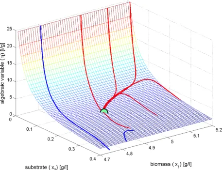
Figure 2: Some trajectories of the system (14) embedded into the QP model (16) The system can be characterized by the following matrices:

A0 =





µ_max 0 0 0 0 0 0 0

0 0 −^µmax_Y 0 0 0 0 0

F

V 0 0 0 ^2µmax_Y ^{K2 2K}_V^{2F µmax}_Y 0





A1 =





0 ^F_V 0 0 0 0 0 0 0 0 0 0 0 0 0 0 0 0 0 0 0 0 0 0



 A2 =





0 0 0 0 0 0 0 0

0 0 0 ^F_V 0 0 0 0

−^2K_V^2F 0 0 0 0 0 0 −^F_V





B =















0 1 1

−1 0 0

1 0 1

0 −1 0

1 2 2

0 2 1

1 1 2

0 0 1















λ0 =





−^F_V

−^F_V 0



 λ1 =λ2 =



 0 0 0



.

(19) The eight quasi-monomials of the QP system model given by the matrices (19) are

x2η, x⁻₁¹, x1η, x⁻₂¹, x1x²₂η², x²₂η, x1x2η², η.

The lower dimensional manifold and some trajectories of the system can be seen on Figure 2. (The inputsXF and SF are held constant.)

2.3 Earlier work on the representation and sta- bility analysis of QP systems

The fundamental works on LV systems was proposed by Lotka [42] and Volterra [65]

which put the LV form into a population biology framework.

From the 90^′sthere are several works about the representation of general nonlin- ear systems having smooth nonlinearities by QP and LV models, e.g. [26], [27] [28].

[27] established the algebraic structure of the class of QP systems. They split into equivalence classes and each class of equivalence is represented by a Lotka-Volterra system.

The other branch of papers are engaged in the stability properties of Lotka- Volterra and quasi-polynomial systems. Local stability analysis of them can be found in [12], where the locally linearized system matrices can be determined directly from the QP or LV system’s parameter matrices.

Several works investigate the global stability of Lotka-Volterra predator-prey models, especially with periodic solutions [59], [43]. However, there are also works on the global stability of quasi-polynomial systems [25], [14]. The main weakness of them is that only small (3-4) dimensional LV systems can be handled with these methods.

An interesting numerical method for their stability analysis is given in [17].

An algorithmic method for finding invariants of quasi-polynomial systems is pro- posed in [51].

On the other hand, the utilization of Lotka-Volterra models for feedback control appears only in few papers [18], or [19], where the positive stabilizing control is proposed only for a subset of LV systems.

Chapter 3

Stability analysis of

quasi-polynomial systems

Global asymptotic stability is a very strong property of all system classes discussed in section1.2and AppendixA.1.1. The global stability analysis of general nonlinear systems (131) is far from being trivial, and results can be obtained only for special system classes.

Based on the fundamental concepts of QP and LV systems presented in chapter2, this chapter draws up own results for the global stability analysis of quasi-polynomial systems. Section 3.1 presents a method for global stability analysis, afterwards, section3.2 generalizes its applicability.

3.1 Global stability analysis using linear matrix inequalities [O4]

This section reformulates the time-decreasing condition of a class of Lyapunov func- tions for Lotka-Volterra systems so that widespread numerical solvers can be used for their global stability analysis.

3.1.1 Global stability analysis

Henceforth it is assumed that x^∗ is a positive equilibrium point, i.e. x^∗ ∈ int(Rⁿ

+) in the QP case and similarly z^∗ ∈int(R^m

+) is a positive equilibrium point in the LV case. For LV systems there is a well known candidate Lyapunov function family [25],[14], which is in the form:

V(z) = Xm

i=1

ci

zi−z_i^∗−z_i^∗ln zi

z_i^∗

, (20)

c_i >0, i= 1. . . m,

where z^∗ = (z^∗₁, . . . , z_m^∗)^T is the equilibrium point corresponding to the equilibrium x^∗of the original QP system (4). The time derivative of the of the Lyapunov function

(20) is:

V˙(z) = 1

2(z−z^∗)(CM+M^TC)(z−z^∗) (21) where C = diag(c1, . . . , cm) and M is the invariant characterizing the LV form (5). Therefore the non-increasing nature of the Lyapunov function is equivalent to a feasibility problem over the following set of linear matrix inequality (LMI) constraints:

CM +M^TC ≤ 0

C > 0 (22)

where the unknown matrix is C, which is diagonal and contains the coefficients of (20). (See Appendix A.4.1 for the properties and solution methods of LMIs.)

Note the similarity of the stability conditions with continuous time LTI systems (127): for a system with state matrix A to be asymptotically stable, there must be positive definite matrices P and Q such that A^TP +P A =−Q (the Lyapunov- equation). If P is a diagonal matrix,A is said to be diagonally stable [33].

It is important to mention that the strict positivity constraint on ci can be somewhat relaxed in the following way [14]: if the equations of the model (4) are ordered in such a way that the firstn rows ofB are linearly independent, thenci >0 for i= 1, . . . , n and cj = 0 for j =n+ 1, . . . , mstill guarantee global stability.

It is examined and proved in [14] and [25] that the global stability of (5) with Lyapunov function (20) implies the boundedness of solutions and global stability of the original QP system (4). It is stressed that global stability is restricted to the positive orthant int(Rⁿ

+) only for QP and LV models, because it is their original domain (see the definition in (4)).

It is also important that the global stability of the equilibrium points of (4) with Lyapunov function (20) does not depend on the value of the vector L as long as the equilibrium points are in the positive orthant [14]. This fact will allow us to place the equilibrium point of the closed loop system during the stabilizing controller design (see section4).

The possibilities to find a Lyapunov function that proves the global asymptotic stability of a QP system can be increased by using time-reparametrization [O4], that is described later in section3.2.

3.1.2 Zero dynamics analysis

The results in this part indicate that a fortunate choice of a QP-type feedback can simplify the dynamics of a closed-loop system in such a way that the number of quasi-monomials may drastically decrease.

Let us consider a SISO input-affine QP-model in the form of (7) with p = 1 and with the simplest output y = xi −w^∗ for some i and w^∗ > 0, i.e. we want to keep the system’s output being equal to a state variable at a positive constant value. Moreover, let us assume that the relative degree of the system equals one and gi1(x) = gi(x) = Qn

j=1x^γ_j^ji, i.e. the input function is of quasi-monomial type (see AppendixA.1.2). Then the output zeroing input is given in the form

u(t) = −Lfh(x)

Lgh(x) =− fi(x) Qn

j=1x^γ_j^ji. (23)

It is seen that the output zeroing input above is in QP-form iff_i(x) is in QP-form.

In order to obtain the zero dynamics (see Appendix A.1.2, or [29]), one has to substitute the input (23) to the state equation (7) to obtain anautonomous system model. It is easy to compute that the resulting zero dynamics system model will remain in QP-form with an output zeroing input in QP-form [O5].

Therefore the stability analysis of the zero dynamics can be investigated using the methods described earlier in section 3.1.1.

The above result can be easily generalized to the case of output functions in quasi-monomial form.

3.1.3 Zero dynamics of the simple fermentation process

In what follows a slightly different version of (14) is examined where the input is the flowrate F. The values of SF, andXF are the constant steady state values of them in (18). The zero dynamics analysis for the fermentation example can be performed e.g. by using the output

y=x2−x^∗₂,

i.e. the centered substrate concentration. The output zeroing input can be easily computed:

F = µmaxx^∗₂V

Y(SF −x^∗₂)x₁η (24)

If the above equations are substituted into the QP-form, one gets the following zero dynamics

˙ x₁ =x₁

µmaxx^∗₂

K2x^∗₂² +x^∗₂+K1 − x^∗₂µmax

Y(SF −x^∗₂)(K2x^∗₂² +x^∗₂+K1)x₁

(25) with QP matrices A^′, B^′ and λ^′ being the following ones:

A^′ =h

−_Y(SF−x^∗_2)(K^x∗2µ2^maxx^∗2

2+x^∗2+K1)

i =

−0.1640 , B^′ =

1

, λ^′ =h _µ

maxx^∗2

K2x^∗2

2+x^∗2+K1

i

=

0.8022 , Hence, the only monomial of the zero dynamics is

X

Note thatthe number of quasi-monomials has been drastically reduced.

In order to study the local stability of the zero dynamics, we first computed the eigenvalue (i.e. the value) of the Jacobian of the zero dynamics at the equilibrium point x^∗₁ that is

−0.8022

Thereafter the feasibility of the LMI (22) was investigated using the LMI Toolbox in Matlab [60] for global stability analysis. The result of the LMI is the following Lyapunov function parameter matrix:

C=

2.7642

Therefore the global stability of the zero dynamics is proved through the QP de- scription. This result is in good agreement with [58] where the stability of the zero dynamics was proved through nonlinear coordinates-transformations.

3.2 Time-reparametrization [O4]

It was shown in [O4], that the significance of time-reparametrization is that it largely extends the possibilities to prove the global stability of a QP system (see e.g. [14]).

As we will see on the examples in section 3.2.4, there are cases when the invari- ant matrix M of the system itself is not diagonally stabilizable (see section 3.1.1), but with an appropriate time-reparametrization, it is possible to find a Lyapunov function of the form (21) for the transformed (reparametrized) model.

3.2.1 The time-reparametrization transformation

Letω = [ω1 . . . ωn]^T ∈Rⁿ. It is shown e.g. in [14] that the following reparametriza- tion of time

dt= Yn

k=1

x^ω_k^kdt^′ (26)

transforms the original QP system into the following (also QP) form dxi

dt^′ =xi m+1X

j=1

A˜i,j

Yn

k=1

x^B_k^˜j,k, i= 1, . . . , n (27)

where ˜A∈Rⁿ×(m+1), ˜B ∈R^(m+1)×n and

A˜i,j =Ai,j, i= 1, . . . , n; j = 1, . . . , m (28)

A˜i,m+1 =λi, i= 1, . . . , n (29)

and

B˜i,j =Bi,j+ωj, i= 1, . . . , m; j = 1, . . . , n (30)

B˜m+1,j =ωj, j = 1, . . . , n. (31)

It can be seen that the number of monomials is increased by one and vector ˜λ is zero in the transformed system.

Special case

A special case of the time-reparametrization or new time transformation occurs when the following relation holds:

ω^T =−bj, 1≤j ≤m, (32)

where bj is an arbitrary row of the B matrix of the original system (4). From (30) and (31) we can see that in this case the j-th row of ˜B is a zero vector. This means

that the number of monomials in the transformed system (27) remains the same as in the original QP system (4) and a nonzero ˜λ vector that is equal to the j-th column ofA appears in the transformed system (for an example, see [14]).

In this case, the ω vector can take only m possible different values (see (32)), therefore the stability analysis of the transformed system reduces to the feasibility check of m different LMIs of the form (22). However, our approach treats the ω vector as part of the unknowns to be determined, therefore from now on we will only consider the generic case discussed in section 3.2.

3.2.2 Properties of the time-reparametrization transforma- tion

The most important properties of the time-reparametrization transformation that are used for analyzing local and global stability are as follows.

Monomials

The set of monomials p1, . . . , pm+1 for the reparametrized system can be written up in terms of the original monomials:

pj = Yn

k=1

x^ω_k^k · Yn

k=1

x^B_k^j,k = Yn

k=1

x^B_k^j,k+ωk, j = 1, . . . , m and

pm+1 = Yn

k=1

x^ω_k^k or using a shorter notation:

pj =r·zj, j = 1, . . . , m p_m+1 =r

where zj is given in (6) and

r= Yn

k=1

x^ω_k^k

Equilibrium points

Since the equations of the reparametrized system (27) can be written as dxi

dt^′ =xi λi+ Xm

j=1

Ai,j

Yn

k=1

x^B_k^j,k

! _n Y

k=1

x^ω_k^k, i= 1, . . . , n (33) and we assume that xi >0, i= 1, . . . , n, it is clear that the equilibrium point x^∗ of the original QP system (4) is also an equilibrium point of the reparametrized system (33).

Local stability

Let us denote the Jacobian matrix of the original QP system (4) at the equilibrium point by J(x^∗). Then the Jacobian matrix of the time reparametrized QP system at the equilibrium point can be computed by using the formula described in [12]:

J(x˜ ^∗) = X^∗·A˜·Z˜^∗·B˜·(X^∗)⁻¹ =r^∗·J(x^∗) = Yn

k=1

x^∗_k^ωk ·J(x^∗), (34) where

Z˜^∗ =diag(p^∗₁, . . . , p^∗_m, p^∗_m+1) , X^∗ =diag(x^∗₁, . . . , x^∗_n)

are the quasi-monomials of the time-reparametrized system and the system variables in the equilibrium point. From (34) one can see that (as we naturally expect) local stability is not affected by the time-reparametrization, because this transformation just multiplies the eigenvalues of the Jacobian by a positive constant r^∗.

Global stability Rewriting (26) gives

dt dt^′ =

Yn

k=1

(xk(t^′))^ωk (35)

from which we can see that t is a strictly monotonously increasing continuous and invertible function of t^′. This means that global stability of the QP system in the reparametrized time t^′ is equivalent to global stability in the original time scale t.

3.2.3 The time-reparametrization problem as a bilinear ma- trix inequality

We denote an n×m matrix containing zero elements by 0^n×m. Let us define two auxiliary matrices by extendingA with a zero column and B with a zero row, i.e.

A¯=

A 0^n×1

∈R^n×(m+1), (36)

and

B¯ =



 B 0^1×n



∈R^(m+1)×n. (37)

Then ˜A and ˜B can be written as

A˜= [A|L] = ¯A+ [0^n×m|L], (38) and

B˜ =









b1+ω^T b2+ω^T

...

b_m+ω^T ω^T









= ¯B +S·Ω (39)

where

Ω = diag(ω)∈R^n×n (40)

and

S =







1 1 . . . 1 1 1 . . . 1

...

1 1 . . . 1





∈R^(m+1)×n (41)

It can be seen from (38) and (39) that the invariant matrix of the reparametrized system is

M˜ = ˜B ·A˜= ( ¯B+S·Ω)·A˜ (42) Therefore the matrix inequality for examining the global stability of the reparametrized system is the following

−C < 0 (43)

M˜^T ·C+C·M˜ ≤ 0 (44)

i.e.

−C < 0 (45)

A˜^T( ¯B^T + ΩS^T)C+C( ¯B+SΩ) ˜A ≤ 0 (46) which clearly has the same form as (22), but with the following set of unknowns:

x=











 x1

x2

...

xm+1

xm+2

...

xm+n+1













=











 c1

c2

...

cm+1

ω1

...

ωn













, (47)

that makes it a BMI (see Appendix A.4.1 for the properties of BMIs). Now we are ready to construct the parameter matrices in the BMI (158) starting with

G¹₀ =G²₀ = 0^(m+1)×(m+1), (48)

G¹_ki,j =

−1, i=j =k

0, otherwise (49)

i, j, k = 1, . . . , m+ 1,

G¹_k = 0^(m+1)×(m+1), k =m+ 2, . . . , m+n+ 1 (50) and

K_kl¹ = 0^(m+1)×(m+1), k, l = 1, . . . , m+n+ 1. (51)

Furthermore, let us introduce the following notations P_k ∈R^(m+1)×(m+1), P_ki,j =

B¯·A˜i,j, i=k

0, i6=k , (52)

i, j, k= 1, . . . , m+ 1 and

Qkl ∈R^(m+1)×(m+1), Q_kli,j =

A˜l−m−1,j, i=k

0, i6=k , (53)

i, j, k = 1, . . . , m+ 1, l =m+ 2, . . . , m+n+ 1.

Then

G²_k =

Pk+P_k^T, k= 1, . . . , m+ 1

0^(m+1)×(m+1), k=m+ 2, . . . , m+n+ 1, , (54) and

Kkl =

Qkl+Q^T_kl, k = 1, . . . , m+ 1, l=m+ 2, . . . , m+n+ 1

0^(m+1)×(m+1), otherwise (55)

k, l = 1, . . . , m+n+ 1.

We note that in certain cases the feasibility of a BMI can be traced back to the feasibility of equivalent LMIs (see [6] or [56]), but in our case it is not possible because of the structural (diagonality) constraint on both of the unknown matrices Ω and C in (46).

3.2.4 Examples

In order to illustrate the above proposed method of finding time-reparametrization transformations for global stability analysis, two simple examples are presented.

Example with a full rank M matrix

Consider a QP system with the following matrices A=

₂

3 −⁸₃

2 3 −⁷₃

≈

0.6667 −2.6667 0.6667 −2.3333

(56)

B = ₂

3 −¹₃

−⁸₃ ¹⁶₃

≈

0.6667 −0.3333

−2.6667 5.3333

(57) L=

2

5 3

≈

2 1.6667

(58) Its equilibrium point of interest is:

x^∗ = [1 1]^T (59)