Generalized total Kalman filter algorithm of nonlinear dynamic errors-in-variables model with application on indoor mobile robot positioning

O R I G I N A L S T U D Y

Generalized total Kalman filter algorithm of nonlinear dynamic errors-in-variables model with application on indoor mobile robot positioning

Hang Yu^1•Jian Wang^2•Bin Wang^3•Houzeng Han^2•Guobin Chang¹

Received: 15 June 2017 / Accepted: 30 September 2017 / Published online: 17 October 2017 ÓAkade´miai Kiado´ 2017

Abstract In this paper, a nonlinear dynamic errors-in-variables (DEIV) model which considers all of the random errors in both system equations and observation equations is presented. The nonlinear DEIV model is more general in the structure, which is an extension of the existing DEIV model. A generalized total Kalman filter (GTKF) algorithm that is capable of handling all of random errors in the respective equations of the nonlinear DEIV model is proposed based on the Gauss–Newton method. In addition, an approximate precision estimator of the posteriori state vector is derived. A two dimensional simulation experiment of indoor mobile robot positioning shows that the GTKF algorithm is statis- tically superior to the extended Kalman filter algorithm and the iterative Kalman filter (IKF) algorithm in terms of state estimation. Under the experimental conditions, the improvement rates of state variables of positionsx,yand azimuthwof the GTKF algo- rithm are about 14, 29, and 66%, respectively, compared with the IKF algorithm.

Keywords Total Kalman filterNonlinear dynamic errors-in-variables modelWeighted total least squaresIntegrated navigation

& Jian Wang

wjiancumt@163.com

1 School of Environment Science and Spatial Informatics, China University of Mining and Technology, Xuzhou 221116, China

2 School of Geomatics and Urban Spatial Information, Beijing University of Civil Engineering and Architecture, Beijing 100044, China

3 College of Geomatics Science and Technology, Nanjing University of Technology, Nanjing 211800, China

https://doi.org/10.1007/s40328-017-0207-7

1 Introduction

An errors-in-variables (EIV) model is different from a Gauss–Markov model, which takes the random errors of both observation vector and coefficient matrix into account. Golub and van Loan (1980) solved the EIV model by the singular value decomposition (SVD) technique, and named the algorithm as total least squares (TLS) for the first time. In the geodetic field, the TLS solution was first applied to coordinate transformation (Liu1983;

Liu and Liu1985; Liu et al.1987). Teunissen (1988) derived the exact solution. Thereafter, studies on the TLS theories and applications are expanded and deepened, such as weighted TLS (Schaffrin and Wieser2008; Shen et al. 2011; Mahboub2012; Amiri-simkooei and Jazaeri2012; Xu et al.2012; Fang2013; Chang2015; Mahboub et al. 2015; Shi et al.

2015), constrained TLS (Mahboub and Sharifi 2013; Fang 2014, 2015; Fang and Wu 2016), outliers processing for TLS (Amiri-Simkooei and Jazaeri2013; Lu et al. 2014;

Wang et al. 2016), TLS for quadratic form estimation (Fang et al. 2015), Bayesian inference for the EIV model (Fang et al.2017), TLS prediction (Li et al.2012; Wang et al.

2017), TLS variance component estimation (Amiri-simkooei 2013, 2016; Xu and Liu 2013,2014; Xu2016; Wang and Xu2016), and TLS precision estimation (Xu et al.2012;

Amiri-Simkooei et al.2016; Wang and Zhao2017).

Obviously, TLS algorithms have been intensively investigated for standard (non-dy- namical) EIV model. The parameter vector is time-independent within the context of the TLS principle. However, the model parameter is non-static in majority of applications.

Kalman filter (KF) algorithm, which is a common algorithm to deal with dynamic model and obtain time-dependent parameters, has been widely used. It was demonstrated in numbers of studies and many different algorithms were investigated, such as the extended KF (EKF) (Gelb 1974), the iterative KF (IKF) (Bell and Cathey1993), Sage–Husa filter (Sage and Husa1969), the particle filter (Liu and Chen1998), unscented KF (Julier et al.

1995), the continuous-discrete KF (Crassidis and Junkins2011). From the viewpoints of applications, the study of KF has involved in many problems, such as integrated navigation (Han et al. 2015,2017; Li et al. 2016), GPS positioning (Xu 2003), and target tracking (Baheti1986).

However, the main challenge faced by the above mentioned KF algorithms is that the random errors of transition matrix of system equations and coefficient matrix of obser- vation equations are ignored. In addition, not too many studies are found that focused on this problem. Schaffrin and Iz (2008) established the dynamic errors-in-variables (DEIV) model for the first time, and a total Kalman filter (TKF) solution within the framework of TLS principle was proposed. Considering the existence of outliers, data snooping tech- nique have been applied to the TKF algorithm by Schaffrin and Uzun (2011). Mahboub et al. (2016) extended the TKF algorithm to a general weighted TKF (WTKF) algorithm which considers a fully correlated dispersion matrix for all of random errors of observation equations. We note that the random errors of transition matrix were not taken into account in these three literatures. Recently, Mahboub et al. (2017a,b) consider the drawback of this kind and present integrated TKF (ITKF) algorithm and constrained ITKF (CITKF) algo- rithm to solve the DEIV model with or without constraints. In the majority of geodetic problems, however, the elements of transition matrix and coefficient matrix are not directly measured variables but are functions of those variables. Therefore, it is necessary to study TKF algorithm under nonlinear DEIV model.

In this contribution, we proposed a generalized total Kalman filter (GTKF) algorithm for nonlinear DEIV model. Although the system equations and observation equations of the nonlinear DEIV model are structurally similar to the nonlinear Gauss–Helmert model

(GHM) (Neitzel2010; Chang2015; Chang et al.2017), the randomness of state vector is considered in this model as well. Considering the nonlinear characteristics of the nonlinear DEIV model, the derivations of the proposed algorithm fully takes advantage of the Gauss–

Newton method of nonlinear least squares, which makes the GTKF algorithm simple in understanding and easy to implement. Then, a first order dispersion matrix of posterior state vector is obtained by using the variance propagation law. Through numerical examples, the performance of GTKF algorithm is illustrated in comparison with EKF algorithm and IKF algorithm.

The remainder of this paper is organized as follows: in Sect.2, the nonlinear DEIV model and GTKF algorithm are formulated. In Sect.3, the iterative scheme of GTKF algorithm is presented. Simulation experiments are illustrated and analyzed in Sect.4.

Finally in Sect.5, conclusions are summarized.

2 Nonlinear dynamic errors-in-variables model and its generalized total Kalman filter algorithm

2.1 Nonlinear dynamic errors-in-variables model

At an epochk, both system equations and observation equations are now expressed as n_k ¼u_kðakeak;n_k1Þ þuk; ð1Þ

y_k¼f_kðbkebk; n_kÞ þeyk; ð2Þ wheren_k1andn_kare them91 time dependent state vectors (unknowns) at epochk-1 andk, respectively,ak is thep91 observation vector contaminated by thep91 random error vector eak,bk is the q91 observation vector contaminated by theq91 random error vector ebk,y_k is the n91 vector of observations, eyk is the n91 random error vector,uk is them91 random system error vector.

The posterior estimaten^þ_k1obtained from the final result at the previous epochk-1 fulfills the following equation

n^þ_k1¼n_k1w_k1; ð3Þ

where the superscript ‘‘?’’ represents the a posterior value,w_k1 is the random error of n^þ_k1.

Assuming that all error terms in Eqs. (1), (2), and (3) are normally distributed, the stochastic model can be described as

wk1

eak

uk

ek

2 66 4

3 77 5

0 0 0 0 2 66 4

3 77 5;

R_k1 0 0 0 0 Qak 0 0

0 0 hk 0

0 0 0 Q_k

2 66 4

3 77 5 0

BB

@

1 CC

A; ð4Þ

whereR_k1,Q_ak, andh_kare the corresponding dispersion matrices ofw_k1,e_ak, andu_k,Q_k is a (n?q)9(n?q) fully correlated dispersion matrix ofek, where

e_k¼ eyk

ebk

; ð5Þ

Q_k ¼ Q_yk Q_ykbk Q_bkyk Q_bk

; ð6Þ

In Eqs. (5) and (6),Q_bk andQ_yk are the dispersion matrices ofebk andeyk,Q_bkyk andQ_ykbk are the cross dispersion matrix betweenebk andeyk.

We further assumed thatwk1,eak,uk, andekare statistically independent of the current and previous state and independent of each other.

2.2 Formulation of generalized total Kalman filter algorithm

The standard Kalman filter algorithm can be performed through two stages, namely, the prediction and the correction. In the prediction stage, the main goal is to give the one-step prediction of the state estimate using the system equations. In the correction stage, how- ever, the observation equations are involved to improve the current (predicted) estimate.

We note that Eqs. (1) and (2) are essentially nonlinear models, the Gauss–Newton method of nonlinear least squares is employed to derive the solution of both two stages.

Since we are going to use the system equations to give the one-step prediction of the state vectorn^_k (the superscript ‘‘-’’ represents a one-step predicted value, the symbol ‘‘^’’

above a variable represents an estimate), the observation equations are not involved in the prediction stage.

The Taylor series expansion is applied to the right-hand side of Eq. (1) at the approximate valuese⁰_a

k andn^þ_k1ofe_ak andn_k1. Thereby, Eq. (1) is now expressed as n_k¼u_kðe⁰_ak;n^þ_k1Þ þGkðn_k1n^þ_k1Þ þHkðeake⁰_akÞ þuk; ð7Þ whereGk¼^oukðe_on^akT^;nk1Þ

k1

ðe⁰_a

k;n^þ_k1Þ,Hk¼^oukðe_oe^akT^;nk1Þ ak

ðe⁰_a

k;n^þ_k1Þ.

Since the prior information ofn_k1is known, the adjustment for the prediction stage can be viewed as the optimization problem with random parameters (Fang 2013; Schaffrin 2009). Therefore, the Lagrange objective function of the prediction stage can be con- structed by combining Eqs. (3) and (7), namely,

UP¼w^T_k1R¹_k1w_k1þu^T_kh¹_k ukþe^T_akQ¹_ak eakþ2k^T₁ðwkn_k1þn^þ_k1Þ

þ2k^T₂ðn_ku_kðe⁰_ak;n⁰_k1Þ Gkðn_k1n^þ_k1Þ Hkðeake⁰_akÞ ukÞ; ð8Þ wherek1andk2denote the Lagrange multipliers. The solution of the Lagrange objective function can be achieved through the following Euler–Lagrange necessary conditions

1 2

oU_P ow_k1

ðw^_k1;n^_k1;n^_k;e^_ak;u^_k;k^₁;k^₂Þ ¼R¹_k1w^_k1þk^₁¼0; ð9aÞ

1 2

oU_P on_k1

ðw^_k1;n^_k1;n^_k;e^_a

k;u^_k;k^₁;k^₂Þ ¼ k^₁G^T_kk^₂¼0; ð9bÞ

1 2

oU_P on_k

ðw^_k1;n^_k1;n^_k;e^_a

k;u^_k;k^₁;k^₂Þ ¼k^₂¼0; ð9cÞ

1 2

oU_P oeak

ðw^_k1;n^_k1;n^_k;e^_a

k;u^_k;k^₁;k^₂Þ ¼Q¹_a

k e^_a

kH^T_kk^₂¼0; ð9dÞ

1 2

oU_P ouk

ðw^_k1;n^_k1;n^_k;e^_a

k;u^_k;k^₁;k^₂Þ ¼h¹_k u^_k k^₂¼0; ð9eÞ

1 2

oU_P ok1

ðw^_k1;n^_k1;n^_k;e^_a

k;u^_k;k^₁;k^₂Þ ¼w^_k1n^_k1þn^þ_k1¼0; ð9fÞ

1 2

oU_P ok2

ðw^_k1;n^_k1;n^_k;e^_a

k;u^_k;k^₁;k^₂Þ ¼ n^_k u_kðe⁰_ak;n^þ_k1Þ G_kðn^_k1n^þ_k1Þ Hkð^e_ake⁰_akÞ u^_k ¼0

ð9gÞ

From Eqs. (9a) to (9f), we can readily obtain the following quantities of the one-step predicted values, namely,

^

w_k1¼0; k^1¼0; k^2¼0; e^_ak ¼0; u^_k ¼0; ð10aÞ n^_k1¼n^þ_k1: ð10bÞ By inserting Eqs. (10a) and (10b) into Eq. (9g), the one-step prediction of state vector n_k is calculated as

n^_k ¼u_kðe⁰_ak;n^þ_k1Þ H_ke⁰_a

k: ð11Þ

We note that the second term in the right-hand side of the above formula can be omitted, since the approximate (initial) valuee⁰_ak ofeakis usually set to zero for numeral calculation.

To achieve the dispersion matrix associated withn^_k, we form the expression for the prior error vector (Brown and Hwang,2012)

e_n

k ¼n_kn^_k

u_kðe⁰_ak;n^þ_k1Þ þGkDn_k1þHkðeake⁰_akÞ þuk ðu_kðe⁰_ak;n^þ_k1Þ Hke⁰_akÞ

¼GkDn_k1þHkeakþuk

¼Gkw_k1þHkeakþuk :

ð12Þ

By using the variance propagation law to Eq. (12), the dispersion matrix of the state estimation error prior to the measurement update is as follow

Qn^_k ¼GkRk1G^T_k þHkQ_akH^T_k þhk: ð13Þ Equations (11) and (13) provide the prior estimate for the correction stage. It should be pointed out that the dispersion matrix of n^_k is in fact a first order approximate matrix which should be updated through iterative process (Amiri-Simkooei et al. 2016; Wang et al.2017).

In similar way, the right-hand members of Eq. (2) is expressed through Taylor series expansion at (e⁰_b

k,n^⁰_k)

y_keyk ¼f_kðe⁰_bk; n^⁰_kÞ þAkðnkn^⁰_kÞ þBkðebke⁰_bkÞ; ð14Þ whereAk¼^ofkðe_on^bkT^;nkÞ

k

ðe⁰_bk;n^⁰_kÞ,Bk¼^ofkðe_oe^bkT^;nkÞ bk

ðe⁰_bk;n^⁰_kÞ.

Regarding the one-step predictionn^_k as the prior expectation ofn_k and taking Eq. (12) into consideration, we can formulate the objective function of the correction stage, namely,

U_C¼ ðe_nkÞ^TQ¹_n^

k e_nkþe^T_kQ¹_k ekþ2K^T₁ðe_nkn_kþn^_kÞ

þ2K^T₂ðy_keykf_kðe⁰_bk; n^⁰_kÞ Akðnkn^⁰_kÞ Bkðebke⁰_bkÞÞ;

ð15Þ

whereK₁andK₂ denote the Lagrange multipliers.

The following necessary conditions must hold for the purpose of optimization, 1

2 oU_C oe_n

k

ð^e_n

k;n^^þ_k;^ek;K^1;K^2Þ ¼Q¹_n^ k

^ e_n

kþK^1¼0; ð16aÞ 1

2 oUC

on_k ðe^_n

k;n^^þ_k;e^_k;K^₁;K^₂Þ ¼ K^₁A^T_kK^₂¼0; ð16bÞ 1

2 oUC

oe_k ðe^_n

k;n^^þ_k;e^_k;K^₁;K^₂Þ ¼Q¹_k e^_k K^2

B^T_kK^2

¼0; ð16cÞ

1 2

oUC

oK₁

ð^e_nk;n^^þ_k;e^k;K^1;K^2Þ ¼e^_nkn^^þ_k þn^_k ¼0; ð16dÞ

1 2

oUC

oK₂

ð^e_nk;n^^þ_k;^ek;K^1;K^2Þ ¼ y_ke^ykf_kðe⁰_bk; n^⁰_kÞ Akðn^^þ_k n^⁰_kÞ Bkð^ebke⁰_b

kÞ ¼0

: ð16eÞ

From Eq. (16c), one obtains

^

ek¼Q_k In

B^T_k

K^2: ð17Þ

By inserting Eq. (17) into Eq. (16e), we have

y_kf_kðe⁰_bk; n^⁰_kÞ Akðn^^þ_k n^⁰_kÞ þBke⁰_bk½In BkQ_k In

B^T_k

K^2¼0: ð18Þ

Therefore, the Lagrange multiplierK^₂ can be calculated as below K^2¼Q¹_g

kðy_kf_kðe⁰_bk; n^⁰_kÞ Akðn^^þ_k n^⁰_kÞ þBke⁰_bkÞ; ð19Þ withQ_g

k ¼½I_n B_kQ_k In

B^T_k

¼Q_ykþB_kQ_bkykþQ_ykbkB^T_k þB_kQ_bkB^T_k.

Furthermore,K^1can be derived by inserting Eq. (19) into Eq. (16b), namely, K^1¼ A^T_kQ¹_g

kðy_kf_kðe⁰_b

k; n^⁰_kÞ Akðn^^þ_k n^⁰_kÞ þBke⁰_b

kÞ: ð20Þ

By taking Eqs. (16a), (16d), and (20) into consideration, we have the following normal equation

ðQ¹_n^

k þA^T_kQ¹_g

kAkÞn^^þ_k ¼Q¹_n^ k

n^_k þA^T_kQ¹_g

kðy_kf_kðe⁰_bk; n^⁰_kÞ þAkn^⁰_kþBke⁰_bkÞ: ð21Þ Then the posterior estimaten^^þ_k can be calculated as

n^^þ_k ¼ ðQ¹_n^ k

þA^T_kQ¹_g

kAkÞ¹ðQ¹_n^ k

n^_k þA^T_kQ¹_g

k ðy_kf_kðe⁰_b

k; n^⁰_kÞ þAkn^⁰_kþBke⁰_b

kÞÞ: ð22Þ

By introducing the matrix inversion lemma (Henderson and Searle1981)

ðVþCZDÞ¹¼V¹V¹CðZ¹þDV¹CÞ¹DV¹ ð23Þ to Eq. (22), an alternative expression ofn^^þ_k is presented as

n^^þ_k ¼n^_k þDn^_k; ð24Þ whereDn^_k ¼Qn^_kA^T_kðQ_gkþA_kQn^_kA^T_kÞ¹ðy_kf_kðe⁰_bk; n^⁰_kÞ A_kðn^_k n^⁰_kÞ þB_ke⁰_b

kÞ.

By substituting Eq. (19) into Eq. (17) and taking Eq. (6) into consideration, one can further obtain the specific expressions of error vectorse^yk,e^bk as follows

e^yk ¼ ðQ_ykþQ_ykbkB^T_kÞQ¹_g

k ðy_kf_kðe⁰_bk; n^⁰_kÞ Akðn^^þ_k n^⁰_kÞ þBke⁰_bkÞ; ð25Þ

^

e_bk ¼ ðQ_bkykþQbkB^T_kÞQ¹_g

kðy_kf_kðe⁰_bk; n^⁰_kÞ A_kðn^^þ_k n^⁰_kÞ þB_ke⁰_b

kÞ: ð26Þ

Applying the variance propagation law to Eq. (24), the precision estimator of n^^þ_k is derived in first order approximation via

Qn^^þ_k ¼Qn^_k Qn^_kA^T_kðQ_gkþA_kQn^_kA^T_kÞ¹A_kQn^_k : ð27Þ

Substituting the posteriori estimaten^^þ_k into Eq. (12), we have

Gk Hk Im

½

^ w_k1

^ eak

^ uk

2 4

3

5 ðn^^þ_k n^_kÞ ¼0: ð28Þ

The formulation of Eq. (28) can be viewed as the conditional adjustment in least squares theory (Zhou et al.2014). Therefore, the estimation of error vectorsw^k1,e^ak, and

^

uk can be estimated as

^ w_k1

e^ak

u^k

2 4

3 5¼

Rk1 0 0 0 Q_ak 0 0 0 hk

2 4

3 5 G^T_k

H^T_k I_m 2 4

3 5Q¹_n^

kðn^^þ_k n^_kÞ: ð29Þ

To achieve the posterior state vector, the above procedure should be implemented iteratively.

3 Iterative scheme of generalized total Kalman filter algorithm

Proposed algorithm for solving generalized total Kalman filter of nonlinear DEIV model is introduced as follows. Note that the superscriptidenotes the iterative index.

1. Epochk=0: input prior estimaten^þ₀ and its dispersion matrixR0; 2. Epochk=k?1: inputak,bk,y_k,Q_ak,hk,Q_k;

3. Set iteration counteri=0:e^^ðiÞ_ak ¼0,e^^ðiÞ_bk ¼0;

4. One-step prediction:n^_k ¼u_kð^e^ðiÞ_a

k;n^þ_k1Þand setn^^{þ ð0Þ}_k1 ¼n^þ_k1,n^⁰_k ¼n^^{þ ð0Þ}_k ¼n^_k; 5. UpdateG^ðiÞ_k ,H^ðiÞ_k ,A^ðiÞ_k ,B^ðiÞ_k at approximate values (^e^ðiÞ_a

k,n^^{þ ðiÞ}_k1,^e^ðiÞ_b

k,n^^{þ ðiÞ}_k );

6. Calculate:

Q^ðiÞ_n^ k

¼G^ðiÞ_k Rk1ðG^ðiÞ_k Þ^TþH^ðiÞ_k Q_akðH^ðiÞ_k Þ^Tþhk ; ð30aÞ

Q^ðiÞ_g

k ¼Q_ykþB^ðiÞ_k Q_bkykþQ_ykbkðB^ðiÞ_k Þ^TþB^ðiÞ_k Q_bkðB^ðiÞ_k Þ^T; ð30bÞ

l^ðiÞ_k ¼y_kf_kðe^^ðiÞ_b

k; n^^{þ ðiÞ}_k Þ A^ðiÞ_k ðn^_k n^^{þ ðiÞ}_k Þ þB^ðiÞ_k e^^ðiÞ_b

k ; ð30cÞ

Dn^^ðiÞ_k ¼Q^ðiÞ_^

n_kðA^ðiÞ_k Þ^TðQ^ðiÞ_g

k þA^ðiÞ_k Q^ðiÞ_^

n_kðA^ðiÞ_k Þ^TÞ¹l^ðiÞ_k ; ð30dÞ

n^^{þ ðiþ1Þ}_k ¼n^_k þDn^^ðiÞ_k ; ð30eÞ

e^^ðiþ1Þ_ak ¼Q_akðH^ðiÞ_k Þ^TðQ^ðiÞ_^

n_kÞ¹ðn^^{þ ðiþ1Þ}_k n^_kÞ; ð30fÞ

w^^ðiþ1Þ_k1 ¼R_k1ðG^ðiÞ_k Þ^TðQ^ðiÞ_^

n_kÞ¹ðn^^{þ ðiþ1Þ}_k n^_kÞ; ð30gÞ

e^^ðiþ1Þ_bk ¼ ðQ_bkykþQ_bkðB^ðiÞ_k Þ^TÞðQ^ðiÞ_g

kÞ¹l^ðiÞ_k ; ð30hÞ

n^^{þ ðiþ1Þ}_k1 ¼n^þ_k1þw^^ðiþ1Þ_k1 ; ð30iÞ

i¼iþ1;

7. Repeat step 5–6 untilDn^^ðiÞ_k Dn^^ði1Þ_k \e (eis a predefined threshold);

¼ ^{ðiÞ ðiÞ}ðA^ðiÞÞ^TðQ^ðiÞþ ^{ðiÞ ðiÞ}ðA^ðiÞÞ^TÞ^{1 ðiÞ ðiÞ}

9. For the next epoch: setn^þ_k ¼n^^{þ ðiÞ}_k andRk¼Qn^^þ_k;

10. Ifk Bt(tdenotes the final epoch) return to step 2, else go to step 11;

11. End.

4 Numerical examples and analyses

Integrated navigation is one of the important implementation techniques for the application of indoor and outdoor positioning. For a moving unit, integrated navigation tries to determine its instantaneous position and attitude by using Kalman filter algorithm. In an outdoor environment, GPS is undoubtedly the primary choice to be implemented due to the global coverage. However, the GPS performance largely suffers from the constraint environments such as urban canyons, multipath error, and large residual atmospheric error.

Therefore, it makes the carrier phase ambiguity resolution difficult to achieve and fur- thermore affects the high-accuracy positioning solutions (Han et al.2017). In regards to an indoor environment, the GPS signal is blocked. Ultra-wideband (UWB) wireless radio system, which operates in the frequency band 3.1–10.6 Hz, has been the focus of attention especially in a closed environment owing to the capacity of strong anti-jamming perfor- mance and immunity of multipath. Nevertheless, the drawback of GPS and UWB is that they are vulnerable to the external environment, such as non-line of sight factor, which makes the two systems cannot be expected to achieve 100% coverage sometimes (Li et al.

2016). Inertial Navigation System (INS) and other sensors, such as odometer and mag- netometer, has the capability of autonomous navigation. The integration of these sensors with GPS and/or UWB can enhance the reliability and availability of an integrated system (Farrell2008; Fan et al.2017).

In this part, an integrated system for a mobile robot experiment in an indoor environ- ment is introduced. Multiple sensors, such as UWB, odometer, and INS, are used to provide range, velocity and angular rate information which contribute to the determination of the final position and azimuth of the robot. Considering the moving unit is on a planar surface, then the height of it is known to behduring the test, namelyz=h. Therefore the position variable can be deemed as two dimensional, and the azimuth angle is the only attitude variable (Farrell2008).

On the basis of the mobile robot experiment, the observation equations and the system equations are essentially nonlinear DEIV model, thus the existing TKF algorithms cannot be employed in this situation. A more reasonable result can be achieved by using the algorithm proposed in this paper.

At an epoch k, the robot kinematics is described by (Farrell2008; Aftatah et al.2016) xk ¼xk1 +ðvkevkÞ sinðw_k1þ ðxkexkÞ DtÞ Dtþux;

yk ¼y_k1 +ðvkevkÞ cosðw_k1þ ðxkexkÞ DtÞ Dtþuy; w_k ¼w_k1þ ðxkexkÞ Dtþuw;

ð31Þ

wherewkdenotes the azimuth angle, Dtdenotes the sampling interval, vkis the velocity measured by odometer and its direction is the corresponding to the moving direction,evkis the error ofvk,xkdenotes the angular rate measured by gyro during the sampling interval Dt,exk is the error ofxk, the symbolsux,uy, and uw represent system errors based on violation of the no-slip assumption.

Equation (31) has the following matrix form

n_k¼n_k1þ ðvkevkÞ M x_kexk

Dtþuk; ð32Þ

withn_k¼½xk yk w_k^T,M¼ sinðw_k1þ ðxkexkÞ DtÞ cosðw_k1þ ðxkexkÞ DtÞ

anduk ¼½ux uy uw^T. At epoch k,

u_k¼n_k1þ ðvkevkÞ M xkexk

Dt; ð33aÞ

ak ¼½vk xk^T; eak ¼½evk exk^T: ð33bÞ Therefore,

Gk ¼ ou_k on^T_k1

!0

¼ ou_k ox_k1

0

ou_k oy_k1

0

ou_k ow_k1

0

; ð34Þ

with_ox^ouk

k1¼

1 0 0 2 4

3 5,_oy^ouk

k1¼

0 1 0 2 4

3 5,_ow^ouk

k1¼

ðv_k1evk1Þ cosðw_k1þ ðxkexkÞ DtÞ ðv_k1evk1Þ sinðw_k1þ ðxkexkÞ DtÞ

1 2

4

3 5Dt.

Hk¼ ou_k oe^T_a

k

!0

¼ ou_k oe_vk

0

ou_k oe_xk

0

; ð35Þ

where^ou_oe^k

vk ¼ M

0

Dt,_oe^ouk

xk ¼

ðvkevkÞ cosðw_k1þ ðxkexkÞ DtÞ Dt ðvkevkÞ sinðw_k1þ ðxkexkÞ DtÞ Dt

1 2

4

3 5Dt.

The observation equations are constructed with the range and azimuth angle information obtained fromls base stations and magnetometer measurement, namely,

p1k

... p_lk w~_k 2 66 64

3 77 75

ep1k

... eplk

ew_k

2 66 64

3 77 75¼

ffiffiffiffiffiffiffiffiffiffiffiffiffiffiffiffiffiffiffiffiffiffiffiffiffiffiffiffiffiffiffiffiffiffiffiffiffiffiffiffiffiffiffiffiffiffiffiffiffiffiffiffiffiffiffiffiffiffiffiffiffiffiffiffiffiffiffiffi ðx¹_se_x¹

sxkÞ²þ ðy¹_se_y¹

sykÞ² q

...

ffiffiffiffiffiffiffiffiffiffiffiffiffiffiffiffiffiffiffiffiffiffiffiffiffiffiffiffiffiffiffiffiffiffiffiffiffiffiffiffiffiffiffiffiffiffiffiffiffiffiffiffiffiffiffiffiffiffiffiffiffiffiffiffiffiffi ðx^l_sex^l_sxkÞ²þ ðy^l_sey^l_sykÞ² q

w_k 2

66 66 64

3 77 77 75

; ð36Þ

wherep1kplkare the l range measurements from the base stations to the tested subject position, w~_k is the azimuth angle obtained from magnetometer measurement, (xs1, - ys1)(xsl

,ysl

) are the positions of base stations which are corrupted by random errors.

Thus, at epoch k,

f_k ¼

ffiffiffiffiffiffiffiffiffiffiffiffiffiffiffiffiffiffiffiffiffiffiffiffiffiffiffiffiffiffiffiffiffiffiffiffiffiffiffiffiffiffiffiffiffiffiffiffiffiffiffiffiffiffiffiffiffiffiffiffiffiffiffiffiffiffiffiffi ðx¹_se_x¹

sxkÞ²þ ðy¹_se_y¹

sykÞ² q

...

ffiffiffiffiffiffiffiffiffiffiffiffiffiffiffiffiffiffiffiffiffiffiffiffiffiffiffiffiffiffiffiffiffiffiffiffiffiffiffiffiffiffiffiffiffiffiffiffiffiffiffiffiffiffiffiffiffiffiffiffiffiffiffiffiffiffi ðx^l_se_x^l

sxkÞ²þ ðy^l_se_y^l

sykÞ² q

w_k 2

66 66 64

3 77 77 75

; ð37Þ

bk¼ x¹_s y¹_s x^l_s y^l_sT

; ebk¼ ex¹_s ey¹_s ex^l_s ey^l_sT

: ð38Þ

The matricesAk andBk can be derived by

Ak ¼ of_k on^T_k

!0

¼ of_k ox_k

0

of_k oy_k

0

of_k ow_k

0

¼ ðD_kÞ⁰ 0l1

012 1

; ð39Þ

and Dk¼ ðDh ¹_kÞ^T ðDⁱ_kÞ^T ðD^l_kÞ^TiT

, Dⁱ_k¼ Dⁱ¹_k Dⁱ²_k

, Dⁱ¹_k ¼

^x

i se_xisxk

ffiffiffiffiffiffiffiffiffiffiffiffiffiffiffiffiffiffiffiffiffiffiffiffiffiffiffiffiffiffiffiffiffiffiffiffiffiffiffiffiffi

ðxⁱ_se_xisxkÞ²þðyⁱ_se_yisykÞ²

q ,Dⁱ²_k ¼ ^y

i se_yisyk

ffiffiffiffiffiffiffiffiffiffiffiffiffiffiffiffiffiffiffiffiffiffiffiffiffiffiffiffiffiffiffiffiffiffiffiffiffiffiffiffiffi

ðxⁱ_se_xisxkÞ²þðyⁱ_se_yisykÞ²

q .

Bk¼ of_k oe^T_b

k

!0

¼ ðD⁰kÞ⁰ 012l

; ð40Þ

withD⁰_k¼

D¹_k 0 0 0 .. .

0 0 0 D^l_k 2

64

3 75.

The superscripts ‘‘0’’ in Eqs. (34), (35), (39) and (40) represent that related expressions are replaced by the corresponding approximate vectors (n⁰_k1,e⁰_ak) and (n⁰_k,e⁰_bk).

Assuming that all the error vectors mentioned above are normally distributed and are generated with the given dispersion matrices.

At initial epoch, i.e. k=0, the dispersion matrix of the random error vector ofn₀is set toR0¼diagð½1 cm²; 1 cm²;ð0:5Þ²Þ. For the system equations, the variance ofevk and exk are set to r²_e

v ¼ ð0:9 m=s)² andr²_ex ¼ ð0:8=sÞ², therefore,Q_ak ¼diagðr²_e

v; r²_exÞ; the dispersion matrix of random system error vector u_k is set to hk ¼diagð½1 cm²; 1 cm²;ð0:1Þ²Þ. For the observation equations, the true positions of base stations (xis

, yis

), where i=1, 2, 3, 4, are given as: (0:5 m; 1 m), (0:5 m; 12 m), (6 m; 12 m), and (6 m; 1 m); The true positions are biased by the random errors with the accuracy of 3 cm; Range and azimuth measurements are biased by the random errors with the accuracy of 6 cm and 0.5°, respectively.

In this experiment, we set the refresh rate of correction stage is 1 Hz while the pre- diction stage is set to 100 Hz, which means that the sampling interval ofDtis 0.01 s. It is thus clear that most of the time only predictions are computed, but corrections are made only when range measurements and azimuth angles are obtained.

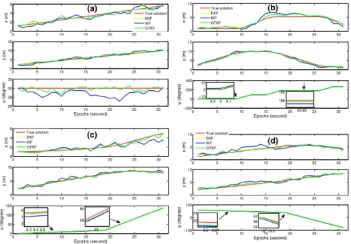
In the application of GTKF algorithm, four different trajectories are simulated in an indoor environment (see Fig.1). We note that the initial true state vector is given as n₀¼½1 m 2 m 30^T for the first trajectory (i.e. Fig.1a), for the second and third trajectories (i.e. Fig.1b, c), we setn₀¼½1 m 2 m 0^T, and for the last trajectory (i.e.

Fig.1d), we setn₀¼½1 m 2 m 60^T.

Since the algorithms proposed by Schaffrin and Iz (2008) and Mahboub et al. (2016) can only deal with linear model situation, in this section, the following three schemes are implemented and compared to show the effectiveness of the proposed GTKF algorithm.

Scheme 1 Extended Kalman filter (EKF) algorithm

Scheme 2 Iterative Kalman filter (IKF) algorithm (Bell and Cathey1993);

Scheme 3 Generalized total Kalman filter (GTKF) algorithm presented in this paper

The threshold for IKF and GTKF are both set to 10^-6. The test results of the above three schemes according to the four simulated trajectories are illustrated in Fig.2. As can be seen from (a–d) of Fig.2, GTKF algorithm (Scheme 3) can achieve the best estimates, which fits the true solution line better in contrast to extended Kalman filter (Scheme 1) and iterative Kalman filter (Scheme 2) algorithms. It should be pointed out that Schemes 1 and 2 ignore the random observational errors in both system equations and observation equations. Nevertheless, GTKF (Scheme 3) algorithm takes all of random errors into consideration. We hence draw the conclusion that GTKF algorithm is more reasonable in theory.

In addition, we run the four simulation experiments based on different trajectories for 10,000 times. The statistics on the absolute errors (i.e. the estimated position and attitude variables minus their counterparts of true values) of each algorithm are presented in Fig.3.

From (a–d) of Fig.3, it is not difficult to find that the IKF algorithm has a slight improvement in comparison with EKF algorithm in terms of statistical absolute errors.

Additionally, the absolute errors obtained by GTKF algorithm are generally smaller than those obtained by the other two algorithms. For the proposed GTKF algorithm, the xvariable is increased by 14%, theyvariable is increased by 29%, and thewvariable is increased by 66% in contrast to the IKF algorithm.

Here, we analyze the computational complexity in terms of the proposed GTKF algo- rithm. The computational complexity of EKF and GTKF is compared. It should be pointed out that the complexity mentioned here is only refers to the time complexity. Table1lists the computational complexity of some basic equations of the proposed GTKF algorithm.

The computational complexity of the one-step prediction [i.e. Eq. (11)] is the same for both EKF and GTKF. Thus, for the sake of simplicity, the complexity of the one-step prediction is not considered. The GTKF algorithm mainly involves Eqs. (30a)–(30i) and Eq. (27). We assume that the average iteration number isT. Hence, according to Table1, the computational complexity of the GTKF algorithm is obtained as

SGTKF¼ ð8Tþ2Þm³þ ð4Tþ4Þn²mþ ð4Tþ6Þnm²þ ðT3Þnm ðTþ1Þm² þ4Tm²pþ4Tmp²Tmpþ3Tmþ8Tn²qþ4Tnq²þ2TnqþTnTp Tqþ ð2Tþ1ÞOðn³Þ þ2TOðm³Þ:

ð41Þ

It is not hard to conclude that the computational complexity of EKF algorithm is (Merwe and Wan2001)

SEKF¼6m³þ8n²mþ10nm²2nm2m²þnþ2Oðn³Þ: ð42Þ From Eqs. (41) and (42), we know that the EKF algorithm and the proposed GTKF algorithm are essentially a linear time algorithm. The computational complexities of EKF and GTKF will be proportional to O(m³Þand/or O(n³Þarithmetic operations. In addition, the average iteration numbers of the GTKF algorithm is T=6.3051 in this example.

Therefore, compared with the EKF algorithm, the complexity of the GTKF algorithm is moderate, especially when considering the modern high-performance computers.

From the iterative scheme of Sect.3, we found that once the error termseak andebkare set to zero, GTKF algorithm will be degraded to IKF algorithm. When the DEIV model is linear and the random errors of transition matrix are ignored, the proposed algorithm will

0 5 10 15 20 25 30

0 2 4

6 (a)

x (m)

0 5 10 15 20 25 30

0 5 10 15

y (m)

0 5 10 15 20 25 30

26 28 30 32

Epochs (second)

ψ (degree)

True solution EKF IKF GTKF

0 5 10 15 20 25 30

0 5

10 (b)

x (m)

0 5 10 15 20 25 30

0 5 10 15

y (m)

0 5 10 15 20 25 30

−200 0 200 400

Epochs (second)

ψ (degree) 8.99 9.1

−10 0 10

23.85 180 185 True solution

EKF IKF GTKF

0 5 10 15 20 25 30

0 2 4 6

(c)

x (m)

0 5 10 15 20 25 30

0 5 10

y (m)

0 5 10 15 20 25 30

0 50 100 150

Epochs (second)

ψ (degree)

8.3 8.4 8.5 5 7 9

23 58 60 True solution

EKF IKF GTKF

0 5 10 15 20 25 30

0 5 10

x (m)

(d)

0 5 10 15 20 25 30

0 5 10

y (m)

0 5 10 15 20 25 30

−100 0 100

Epochs (second)

ψ (degree)

8.2 8.24 52 53

19 19.2 34 38 42 True solution EKF IKF GTKF

Fig. 2 The position and attitude solutions of different algorithms:a–dare the solutions based on the simulated trajectory of Fig.1a–d, respectively