REGULATION OF METABOLIC MODELS MATHEMATICAL 18

(1)

Symposia Biologica Hungarica 18

MATHEMATICAL MODELS

OF METABOLIC REGULATION

Akadémiai Kiadó, Budapest

(2)

M A THEM ATICAL M O D ELS O F M ETA B O LIC

R E G U L A T IO N Edited by

T. KELETI and S. LAKATOS (Sym posia Biologioa H u n g aric a

18)

T his volum e com prises th e p ap ers delivered a t th e F E B S A dvanced Course N o. 27 held a f te r th e 9th M eeting o f th e F ed era tio n o f E u ro p e a n B io

chem ical Societies in 1974. T he re p o rts o f th e le ctu re rs give an overall p ic tu re o f th e p re se n t s ta te o f th e ir research fields including so far unpu b lish ed results.

T he p ap ers d eal w ith th e b io chem ical aspects o f th e re g u latio n o f m etabolic p a th w a y s an d th e possibilities o f m a th e m a tic al m odelling o f su ch sy s

tem s. Special a tte n tio n is d e voted to th e k e y enzym es an d enzym e system s, f u rth e r to th e in te ractio n o f th e se enzym es a n d m em branes as well as to th e biochem ical, biophysical an d m a th em atical descriptions o f k i

n etic analysis o f th e m etabolic processes.

T he volum e is recom m ended for those ac tiv e ly engaged in biochem ical a n d b iophysical re search b u t it m a v be useful also for m ath em atician s, p h y s icists, biologists a n d m edical w orkers w ho a re in te re ste d in th e c u rre n t problem s a n d tre n d s o f m etabolic regulation.

AKADÉMIAI KIADÓ Publishing House of the Hungarian Academy of Sciences

BUDAPEST

(3)

Symposia Biologïca Hungarica

18

(4)

S y m p o s i a Biologica H u n g a r i c a

R e d i g i t

T. K E L E T I e t S. LA KA TOS

Vol. 18

A K A D É M IA I K IA D Ó , B U D A PE S T 1976

(5)

MATHEMATICAL MODELS OF

METABOLIC REGULATION

E d ite d by

T. KELETI

Enzymology Department, Institute of Biochemistry, Hungarian Academy of Sciences, Budapest, Hungary

and

S. LAKATOS

Enzymology Department, Institute of Biochemistry, Hungarian Academy of Sciences, Budapest, Hungary

A K A D É M IA I K IA D Ó , B U D A P E S T 1976

(6)

The F E B S A dvanced Course No. 27 was held a t Dobogókő, 1—5 Septem ber, 1974

ISBN 963 05 0919 9

(7)

LIST OF CONTRIBUTORS

Ac h il l e s, W . I n s titu te o f P hysiological C hem istry, F ried rich Schiller U niversity, J e n a , G D R

Be l l m a n n, K . C entral I n s titu te o f C ybernetics an d In fo rm a tio n Processes, A cad.

Sei. G D R, 1199 B erlin-A dlershof, R u d o w er Chaussee

Bö t t n e r, R . C entral I n s titu te o f C ybernetics an d In fo rm a tio n Processes, A cad. Sei.

G D R , 1199 B erlin-A dlershof, R udow er Chaussee

Bu b l it z, R . I n s titu te o f P hysiological C hem istry, F ried rich Schiller U niv ersity , Je n a , G D R

Cu m m e,G. I n s titu te o f Physiological C hem istry, F ried rich Schiller U n iv ersity , J e n a , G D R

En d r é n y i, L. D e p a rtm e n t o f P harm aco lo g y an d D e p a rtm e n t o f P re v e n tiv e M edicine a n d B iostatistics, U n iv ersity o f T oronto, T oro n to M5S 1A8, C an ad a

Fa j s z i, Cs. I n s titu te o f Biophysics, Biological R esearch C enter o f th e H u n g a ria n A cadem y o f Sciences, Szeged, H u n g ary

Fr u n d e r, H . I n s titu te o f P hysiological C hem istry F ried rich Schiller U n iv ersity , Je n a , G D R

He in r ic h, R . H u m b o ld t-U n iv e rsitä t zu Berlin, I n s titu t fü r physiologische u n d b io logische Chemie, B erlin, D D R

Ho r n, A. I n s titu te o f P hysiological C hem istry F ried rich S chiller U n iv ersity , Je n a , G D R Ke l e t i, T. E nzym ology D ep a rtm en t, In s titu te o f B iochem istry, H u n g a ria n A cadem y

o f Sciences, B u d ap est, H u n g ary

Kn ij n e n b u r g, A. C entral I n s titu te o f C ybernetics an d In fo rm a tio n Processes, A cad.

Sei. G D R 1199 B erlin-A dlershof, R udow er Chaussee Ku r g a n o v, B. I. I n s titu te for V itam in R esearch, Moscow, U SSR

Ne u m a n n, H . C entral I n s titu te o f M olecular Biology, A cad. Sei. G D R , B erlin-B uch, L indenberger W eg

Pr a j d a, N . L a b o ra to ry for E x p e rim e n ta l Oncology an d D e p a rtm e n t o f P harm aco lo g y , In d ia n a U n iv ersity School o f M edicine, Indian ap o lis, In d ia n a , U SA 46202 Ra p o p o r t, T. A. A kadem ie d er W issenschaften der D D R , Z e n tra lin stitu t für M oleku

larbiologie, B ereich B ioregulation, B erlin-B uch, D D R

Re ic h, J . G. Z e n tra lin s titu t fü r M olekularbiologie, B ereich M ethodik u n d Theorie, B erlin-B uch, D D R

7

(10)

Ri c a r d, J. L ab o rato ire de Physiologie Cellulaire V égétale Associé au C. N. R. S.

U n iversité d’Aix-M arseille, C entre de L um iny, 13288 M arseille Cedex 2. F ran ce We b e r, G. L ab o ra to ry for E x p erim e n ta l Oncology an d D e p a rtm e n t o f Pharm acology,

In d ia n a U n iv ersity School o f Medicine, In dianapolis, In d ian a , USA 46202 Wil l ia m s, J . C. L a b o ra to ry for E x p erim e n ta l Oncology an d D e p a rtm e n t o f P h a rm a

cology, In d ia n a U n iv ersity School o f Medicine, Indianapolis, In d ian a , USA 46202 Wr ig h t, B. B oston B iom edical R esearch I n s titu te , B oston, Ma. USA

(11)

I. MODELLING OF THE KINETIC AND REGULATORY BEHAVIOUR

OF ENZYMES

(12)

(13)

Sym p. Biol. Hung. 18, pp. 11— 30 (1974)

STATISTICAL PROBLEMS OF KINETIC MODEL BUILDING L. ENDRÉNYI

Department of Pharmacology and Department of Preventive Medicine and Biostatistics, University of Toronto, Toronto M5S 1A8,

Canada

ROLE AND LIMITATIONS OF STATISTICS IN MODEL BUILDING

Statistical methods are utilized with increasing frequency for the evaluation of quantitative data. They are, of course, often very useful.

Indeed, one aim of this brief review is to call attention to their applicability. At the same time, thoughtless application of any useful technique or method can lead to misinterpretations, exercises in futility and dangerous misunderstandings. Therefore, it may be worthwhile to delimit the place of statistical procedures in kinetic and in general, in

quantitative investigations.

Certainly, it is pointless to ask for the statistical evaluation of data when the conclusions are obvious anyway. Thus, the presence or absence of "statistical significances" can be meaningless when

phenomena are clearly observed. After all, the use of statistics in the biological sciences is only a fairly recent custom, and many very valuable observations have been made and conclusions reached without resorting to such "sophisticated" procedures.

Thus it may not be useful to apply statistical methods for the evaluation of data which are practically error-free or involve only very small errors. Similarly, statistics can be of little help in the presence of very scattered, poor observations. Artificial manipulation or

"massaging" of such data can only mislead an unwary investigator.

Statistical methods are applied most fruitfully with moderately scattered data. They can be used very effectively and efficiently indeed in the vast range of studies admitting this condition.

Substantial information can frequently be extracted which would be inaccessible to other methods.

Nevertheless, like any technique, statistical analysis of experimental data has its limitations and will not provide an all-embracing solution, a panacea to all kinetic modelling problems.

Consequently, it is a dangerous practice (seen with increasing frequency in the literature) to rely for analysis solely on numerical, statistical solutions and computer printouts. These methods should not be used blindly but with great deal of common sense, ideally in conjunction with traditional procedures, including linearizations and replots which frequently provide at least guidance for the interpretation of the observations. The continuous interplay between statistical computations and graphical evaluations is very strongly recommended.

11

(14)

STRATEGY OF MODEL BUILDING

A scientific investigation is performed presumably in order to learn about a biological, chemical, physical, etc. phenomenon. Certainly, at the conclusion of the study, and possibly at its commencement, assumptions, hypotheses are made which characterize the phenomenon. As a result, a biological, chemical, physical, etc. model is visualized.

HYPOTHESIS

BIOLOGICAL MODEL

OBSERVATIONS

MATHEMATICAL MODEL

E X P E R IM E N T

Fig. 1. General strategy of model building.

For the purpose of quantitative studies, this model can be described in mathematical terms. The resulting expressions, the mathematical m od e l s , can characterize simply straight-line, linear relationships or they can be much more complicated, such as a system of differential equations.

The hypothesis of a mathematical model should be justified and characterized on the basis of observations. Usually experiments are designed, performed and analyzed for this purpose. Therefore, the experiment and its analysis have two main purposes: First, the validity of the mathematical model must be evaluated, for example, by testing the linearity of a supposedly straight-line relationship. Adoption of a mathematical model implies also conclusions about the validity of the biological model, since computations based on the observations at least do not argue against it.

Once a model is tentatively accepted, interest centers on the evaluation of its constants. Actually in practice, the computations involving model identification and parameter estimation are usually pursued simultaneously. In principle, however, these two processes should be carefully distinguished not only in order to clarify the principal purpose of the investigation (a very important requirement, not always considered), but also because the efficient experimental design for estimations and for validity tests may not be the same (Hill, Hunter and Wiehern, 1968).

The repeated cycle between model hypothesis and experimentation, in

cluding the design and analysis of the latter, is a basic characteristic of scientific investigations (Box and Hunter, 1962). It is illustrated in Fig. 1.

As an illustrative example, the Briggs-Haldane model for simple enzymic reactions will be considered:

(15)

E + S ES E + P

The corresponding mathematical model, the Michaelis-Menten equation, describes the relationship between the reaction velocity (v) and the substrate concentration (c):

v Vc

К +

m c

The expression characterizes a rectangular hyperbola with two constants:

The maximal velocity (V) and the so-called Michaelis constant (K^).

In order to characterize a particular enzymic system, an investigator performs an experiment with N observations. The observed reaction

velocities,

vi

Vci К +

m

i = 1,2,...,N,

are not free of experimental errors (e^) which are superimposed on the unknown true velocities, so that

v . = v + e .

i 1

As will be described later, the model can be analyzed by several methods. These include the various well-known linearizations of the hyperbola which can be utilized to test the validity of the mathematical, and therefore of the biological model (the Michaelis-Menten equation and Briggs-Haldane mechanism, respectively). This approach (which is, as will be seen, not necessarily the best one) relies on the evaluation of the actually observed linearity of the transformed observation.

The linearizations and the corresponding plots can be utilized also for the estimation of the two parameters. This is a customary procedure but, as will be seen, certainly not a recommended one.

PURPOSES OF MODEL BUILDING

Investigations into the characteristics of models (i.e., model building studies) are pursued for two main reasons. The first driving force is man's quest for knowledge, his search for insight into manifestations of nature.

Therefore, he wishes to establish the features of various phenomena, to describe the mechanisms of processes, including those of chemical reactions, and to evaluate the magnitude of natural constants, including those of equilibrium and rate constants.

The second principal motivation for developing models lies in their utilization. For example, they can be applied for interpolation, and to some extent even for extrapolation and, therefore, for prediction.

But merely for prediction we do not necessarily require models based on natural, e.g. biological foundations. In principle, superficial but appropriately descriptive and sufficiently accurate characterizations would be quite satisfactory. Thus, we can distinguish two kinds of models: Those fundamentally relying on natural principles, including those based on mechanisms of processes (mechanistic or

deterministic models) , and those in which such foundations are more tenous or perhaps even entirely absent. Such empirical models may simply involve, in part or entirely, past experience concerning the properties and behaviour of the investigated system.

13

(16)

The mathematical form of a mechanistic model reflects, of course, features of the underlying natural models. An example is the already mentioned Michaelis-Menten equation. In contrast, empirical models may be described by very simple expressions, such as polynomials which may contain coefficients having no physical meaning at all.

The methodology of statistical analysis of the experiment, in particular that of parameter estimation, follows the division between the two model types. As will be indicated in greater detail later, parameter estimation must be performed with much greater care when insight into a model is desired than with the interest of the investigator restricted merely to the prediction of responses.

FACTORS AFFECTING MODEL IDENTIFICATION AND PARAMETER ESTIMATION Quite naturally all investigators want to obtain information as reliably and as efficiently about the studied models as possible. It is, therefore, necessary to consider the main factors influencing the

effectiveness of model validity tests and of parameter estimation. These include

i) the properties of the experimental error;

ii) the experimental design; and iii) the method of evaluation.

The development and evaluation of models is assisted very

substantially if the investigator pays thorough attention to these factors.

In order to emphasize this important point, the recommended considerations and actions are summarized in Table 1. They will be analyzed now in some detail.

Table 1.

Investigators' approach to factors influencing the effectiveness of model building

Factor Action expected of

investigator Experimental error

Constant absolute error?

Constant relative error?

Recognizes characteristics

Experimental design

Number of observations Range of observations Scaling of observations

Carefully chooses optimum

Method of analysis

Nonlinear regression Weighting?

Linear transformations, graphs

Selects principal method Uses combination

(17)

CHARACTERISTICS OF THE EXPERIMENTAL ERROR

It is assumed in most model building procedures, including those based on the methods of least squares, that the experimental errors are present only in the dependent but not in the independent variables, that they are random and have constant variance, independently of the magnitudes of the variables and that, for the evaluation of statistical significance tests and confidence limits, they follow the normal, Gaussian distribution.

Failure of one or more of these assumptions can lead to inadequate and misleading results.

Deviations from the assumption of normally distributed errors Are rather difficult to detect. For example, plots of the estimated errors (the residuals, to be discussed later) in cumulative normal grids require a large number of observations (Daniel and Wood, 1971). Fortunately, results of analyses are believed to be quite robust against moderate divergences from normality.

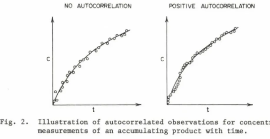
The assumption of randomness implies that the various observations and their errors are independent of each other, with no correlations among them. This is often reasonably correct in the case of binding or steady- state rate equations. However, as illustrated in Fig. 2, correlations

NO AUTOCORRELATION POSITIVE AUTOCORRELATION

Fig. 2. Illustration of autocorrelated observations for concentration measurements of an accumulating product with time.

between consecutive time-dependent observations can be very high. The consequences of such autocorrelations (which are estimated by the

corresponding observed serial correlations; Kendall and Stuart, 1966) are generally small (Suranyi, 1973) and therefore neglected. Still, it is worth pointing out that apparent serial correlations can be brought about by unusual, outlying data points. Therefore, detection of outliers is aided by the analysis of error correlations (Reich, 1974).

Among the characteristics of experimental errors, the assumption of their constant variance is particularly important since divergences from its validity have very strong effects on the outcome of model identification tests and parameter estimations. Fortunately, as we shall see later,

deviations from this condition can be fairly conveniently evaluated and corrections can be made for these.

Very frequently, the absolute magnitude of the experimental error tends not to remain the same in the whole range of the investigation

(corresponding to the assumption of constant error variance) but increases proportionately with the value of the response (the reaction velocity in kinetic studies). Actually, in this case, the ratio of the error to the response, i.e. the relative error, i.e. the coefficient of variation remains

15

(18)

constant, which is a very usual condition.

Therefore, it is important that the investigator should make a

serious effort to recognize the trend in the error behaviour (cf. Table 1).

In particular, he should evaluate whether the absolute or the relative Table 2.

Principal types of error behaviour

Absolute error

°i

Relative error V v i

Constant Decreases with v

Increases with v Constant

v^: Reaction velocity predicted at i-th observation.

a^: Expected standard deviation of i-th observation.

error remains constant in his experiment (Table 2). Residual plots, which will be described later, can be applied to advantage for this purpose.

EXPERIMENTAL DESIGN

The design of the experiments has very strong influence on the effectiveness of model identification (Box and Hill, 1967) and parameter estimation (Box and Lucas, 1959). Therefore, whenever possible, the investigator should select the most efficient design for the task

(cf. Table 1). In particular, the components of the design should be considered, including

i) the number of observations (N);

ii) the range of the measurements; and

iii) the arrangement or spacing of the independent variable.

Increasing the number of observations improves, of course, the effectiveness of all aspects of model building (when correctly executed, see later). The final number will be the result of a compromise between the desired excellence of the results and the increasing expense in time, effort and funds.

The effect of the observational range on the outcome of the model building may be more surprising since efficiency can frequently be

improved not by expanding but, on the contrary, by restricting the range of experimentation. For example, in hyperbolic kinetic or binding studies, with constant absolute observational errors, the effectiveness of parameter estimation is improved when the measurements are restricted to relative velocities not lower than 0.2 or to fractional bindings not lower than 0.4

(Endrényi and Kwong, 1972).

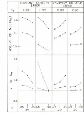
This is illustrated in Fig. 3. With constant absolute error, both the precision and the bias of the parameters improve when the range of the observations is restricted at the lower end. In contrast, with constant relative errors such confinement would be ruinous since, under this error condition, the precision and accuracy of the estimated parameters improve by widening the range of observations.

(19)

Fig. 3. Effect of experimental design on the precision and accuracy of kinetic parameters which are estimated by nonlinear regression.

Each point represents the averaged result of 100 computer

simulated experiments with N=5 observations, with the concentrations uniformly spaced, and true parameters V = 1.0 and Кщ = 1.0.

Either constant absolute error of = 0.10 or constant relative error of = 0.20 v^ was assumed in the experiments. In the latter case the parameters were evaluated by weighted nonlinear least-squares calculations.

The open circles show estimates of V, the dark triangles refer to those of Кд,.

The lower half of the diagram provides a measure of the bias (deviation from the true value of unity) in the average value of the estimated parameters. The upper half illustrates MSE, the mean square parameter error averaging the variances of the estimated parameters, which is a measure of their precision

(reproducibility).

The smallest and largest relative velocities, vi and V5, are indicated on the bottom and at the top of the diagram, respectively.

Such considerable contrasts between effective experimental designs emphasize again the great importance of the necessity for recognizing the error behaviour of the observations.

Restricting the range of observations does not agree with the usual conduct of the investigations. For the explanation we have to return to the already stressed two main purposes of mechanistic model building:

Model identification and parameter estimation. The desirability, under certain conditions, of restricting the range of measurements has been concluded for the efficient evaluation of the two parameters. This has

2 17

(20)

implied that we have been reasonably certain of the applicability of the Michaelis-Menten equation. If, however, the appropriateness of the model is to some extent in question then readings have to be obtained also at lower concentrations in order to evaluate, for instance, the absence of

sigmoidicity. Ideally again a compromise should be reached in which some observations aim at demonstrating the applicability of the hyperbolic model while the remaining ones evaluate the parameters in the most efficient way using the most effective design for this purpose.

METHOD OF ANALYSIS

By far the most frequently technique of statistical model building is the method of least squares since, as we shall see later, it has many favourable properties.

Initially, an arbitrary set of values is selected for the model parameters. From these, on the basis of the model, responses (reaction velocities) are calculated which are compared with the observed responses.

The basis of the comparison is the so-called sum of squares (SS) which is the sum of the squared differences between the observations (v^) and the corresponding values predicted from these models (v^),

ss =

By selecting new values for the parameters, the predicted responses and, therefore, the sum of squares can be recalculated. As the best values, those parameters will be chosen which yield the smallest of all possible sum of squares. These estimated, least-squares parameters are designated by a "hat" mark over them.

In the example of the Michaelis-Menten equation, the two parameters, V and Ид,, can be systematically varied to obtain their least-squares values,

$ and ÍCjjj, corresponding to the minimum sum of squares, VCf

SS = E(Vl - ---)2

As mentioned above, corrections can be made if changes in the error variance are recognized. In this case, the sum of squares is weighted before minimization,

SSw “ r w i (vi - v i)2

with weights (w^) inversely proportional to the variance of the error,

If, for example, the relative error of observations is constant throughout the range of experimentation then the standard deviation is proportional to the response (which is estimated by the predicted response),

ai oc _V

i

(21)

and the weight is inversely proportional to the square of the predicted response,

w a 1/v2 Therefore, the minimized sum of squares is now

ssw - S(V± - v±)2 / 02

It must be emphasized concerning the selection of weights that they should be based on a scheme of error behaviour (e.g., constant absolute or constant relative errors) involving the entire set of observations since this gives reasonable confidence in their validity. The weights should not rely merely on replicate readings obtained at a given experimental condition

(at a given set of independent variables; Ottaway, 1973) since their reliability would be very limited. The reason for this, in statistical language, is that they would be based on very few degrees of freedom.

The calculations, based on the method of least squares are quite straightforward if the model is linear in all of its parameters since, in this case, the parameters and the corresponding minimum sum of squares can be computed from explicit formulas. If, however, the model is not linear with respect to all of its parameters, then the sum of squares must be minimized by iterative calculations. Naturally, such nonlinear regression analyses are facilitated by the use of computers.

The Michaelis-Menten model is linear in one of its parameters, V, but not linear with respect to the other, К . Thus, its analysis should involve nonlinear regression computations (Wilkinson, 1961; Cleland, 1963, 1967; Bliss and James, 1966).

Traditionally, evaluations of the Michaelis-Menten equation have been based on one of its linear transformations. These have been used both for model identification and parameter estimation. Their analysis can be purely graphical or again the method of leastj Squares may be applied.

Consequently, as will be discussed, there is a selection among the analytical methods (which is in fact much wider). Therefore, the

investigator can and should choose the best, most effective procedure among these (cf. Table 1). An even more preferable approach, especially in studies of complex systems, utilizes more than a single procedure. Without

exception, each of these has limitations. Reliance on only a computational or solely on a graphical method can be very dangerous. Consequently, mutual confirmation of the conclusions and quantitative results by a variety of methods is very desirable. This procedure is strongly recommended and urged.

PROBLEMS OF NONLINEAR REGRESSION COMPUTATIONS

To recapitulate, in nonlinear regression analysis the model

parameter values are varied until they yield the smallest sum of squares value. Therefore, we are searching for an absolute minimum

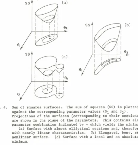
on a surface of sum of squares plotted against the appropriate parameter values (Fig. 4).

Several computational schemes have been devised which explore the surface, seeking its minimum. The task of such optimization routines is easy when the surface itself is smooth with nearly ellipsoidal sections indicating almost linear characteristics (Fig. 4a). At other times, however, the surface is bent, elongated, "banana-shaped" (Fig. 4b). The search for

2* 19

(22)

Fig. 4. Sum of squares surfaces. The sum of squares (SS) is plotted against the corresponding parameter values (6^ and 0£ ) . Projections of the surfaces (corresponding to their sections) are shown in the plane of the parameters. This contains also the parameter combination indicated by + which yields the minimum SS.

(a) Surface with almost elliptical sections and, therefore, with nearly linear characteristics. (b) Elongated, bent, strongly nonlinear surface. (c) Surface with a local and an absolute minimum.

its minimum is much more difficult, often frustrating. Still other surfaces have more than one minimum (Fig 4 c ) . Their exploration may falsely stop at a local minimum instead of going on to the true absolute minimum.

There are many general and very useful computer programs and packages attempting to remedy these difficulties (for example, Cornish-Bowden and Koshland, 1970; Atkins, 1971; Reich et al., 1972, for kinetic purposes).

All # of them can conveniently be used for most model building problems. However, none of the routines can solve all difficult situations and none can claim to provide the all-round best procedure.

The problem of multiple minima was already mentioned. As a result, the user is never quite certain of reaching the smallest sum of squares, the absolute minimum. This problem of uniqueness can be overcome by starting the exploration of the surface at several points, that is, by assuming initially several different sets of parameters. They should yield repeatedly the same final set of constants.

It should be emphasized that the assumed error behaviour with the corresponding weights determines the shape of the sum of squares surface.

Consequently, the minimum and the least-squares parameters are fixed by

(23)

supposing, for example, the condition of constant absolute or constant relative error but they do not involve the assumption of any kind of error distribution.

RESIDUAL PLOTS, TEST OF ERROR BEHAVIOUR

After reaching the minimum, the various assumptions made earlier must be tested. Very important among these is the hypothesis of random errors having constant variance which is evaluated most frequently by the very useful residual plots. These contrast (weighted) residuals with the various independent variables, with the observed or the predicted response or with the time sequence of the observations (Draper and Smith, 1966;

Daniel and Wood, 1971, pp. 27-32). Systematic deviations, nonrandom trends indicate the inadequacy of the assumed m o d e l .

The weighted residuals are (Box and Hill, 1974)

» w^ (observed response - predicted response)

= J V (v^ - v^)

for reaction velocities.

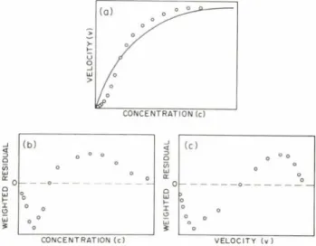
For example, if a hyperbola is fitted to kinetic data which actually characterize a system with positive deviations from hyperbolic behaviour

(for instance, a system described by a sigmoidal rate curve) then systematic

Fig. 5. Residual plots demonstrating the inadequateness of an assumed model, (a) Hyperbolic rate curve fitted to observations involving a nonhyperbolic kinetic system. (b) Residuals plotted against the independent variable or (c) against the observations show systematic trends, i.e., deviations from randomness.

trends are noted in the observed residual plot (Fig. 5). Advantages of the plot include its being illustrative and very sensitive. This is useful since, for example, positive nonhyperbolicities are not necessarily indicated by the appearance of sigmoidicity (Ainsworth, 1968; Endrényi, Chan and

21

(24)

Weng, 1971).

Residual plots can be applied not only in order to aid model identification, but also to characterize the observational error and, in particular, to distinguish between the two main types of error behaviour.

PLOT

CONSTANT ABSOLUTE ERROR сг - CONSTANT

CONSTANT RELATIVE ERROR

< V v -CONSTANT

RATE

C U R V E ^V

/ y ő ' "

Ь А /

( O f w

V

[ / * .

c c

RESIDUALS FROM MINIMISING

UNWEIGHTED

s s

e 0

О ’ о °

e 0

° о ° V

о о

о V *

RESIDUALS FROM MINIMISING

WEIGHTED

s s

e

0

ч e

0 j

1

0

•o

1 °°

_ _

о о у

✓

о V

- о ° о

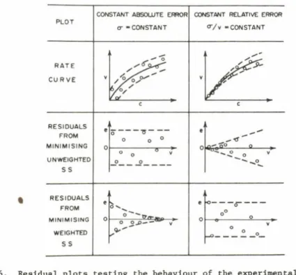
Fig. 6. Residual plots testing the behaviour of the experimental error.

The two rate curve plots illustrate the two main types of error behaviour: constant absolute error or constant relative error. If a rate equation is fitted to the data by assuming the former error condition then the residuals conforming with the error behaviour show randomness in a horizontal band. Conflict with the

true error behaviour is revealed by a widening belt. Similarly, randomness is indicated when the curve-fitting based on the assumption of constant relative errors corresponds to the true error properties, while a narrowing error band suggests

disagreement with the error hypothesis.

As illustrated in Fig. 6, a given set of observations can be fitted successfully by least-squares curves based on the assumption constant absolute and then by constant relative error. The assumption corresponding to the true error behaviour yields a plot in which the residuals with the appropriate weights are randomly placed in a horizontal band. In contrast, by using weights not corresponding to the true error behaviour,

characteristically non-random plots are obtained. For instance, assuming in the computations constant relative errors when, in fact, the absolute

magnitude of the errors tends to remain constant, the band of residuals narrows. The reverse situation is indicated by exactly the opposite

pattern: If a system is actually characterized by constant relative errors but the data are fitted by assuming constant absolute errors, then the residuals are in a wedge-shaped, widening zone.

(25)

Various formal schemes have been proposed for the evaluation of error behaviour. These include the use of transformations (Box and Cox, 1964), the regression of the absolute value of the residuals (e) against the response (Glejser, 1969), and an F-test comparing the sum of the

squares of the last residuals in an ordered sequence against the sum of the squares of the initial residuals (Goldfeld and Quandt, 1965),

, 2 . 2

(eN + eN-l + -

.) / (ej +

e

2 2 +...)

Kwong (1972) compared these methods and concluded that the F-test was most powerful. He recommended that the first and last m points of the sequence should be included in the test where m is the integer part of (N+3)/4 . For example, with N=10 observations, m = I n t (13/4) = 3 , and

_ / 2 j 2 2 -. / / 2 , 2 . 2.. F = (e10 + e 9 + e8 1 (el + e2 + e3 )

The performance of the test has not been compared with those of the residual plots. Their use is very strongly recommended both for model identification and for the evaluation of error behaviour.

MODEL IDENTIFICATION

We return now to the main tasks of model building: Model identification and parameter estimation for the characterization of mechanistic models and for prediction.

Some approaches have already been mentioned which are useful for the identification of models. They included the application of residual plots which could indicate incompatibility with the assumed model.

Serial correlations were noted to indicate disagreement with some of the assumptions made or to suggest the presence of outliers.

Some other useful criteria have been summarized by Bartfai and Mannervik (1972). These include the success of nonlinear regression

computations and examination of the estimated parameter values. Slowness or failure of the computer routine to converge, from several initial points, to a minimum raises suspicion about the validity of the model. Similarly, doubts are caused by unreasonable values of the estimated parameters or by their relatively large standard errors. (It has occasionally been suggested that negative parameter estimates, which could not characterize kinetic or equilibrium constants, would be restricted simply by constraining the range of accessible values. It is firmly believed that this approach would merely evade but not solve the problem. As we shall now see, negative estimates of constants actually call attention at their dispensability.) Convergence problems, unreasonable parameter values or large errors are often manifestations of the same problem: The presence of redundant parameters.

Eliminating these from the model will frequently cure the anomalies (Box and Jenkins, 1970; Reich and Zinke, 1974). Redundance is indicated also when the information matrix has very small eigenvalues.

The variance of the observational errors estimated from the minimum sum of squares provides further evidence of the adequacy of the model. If an independent measure of the errors is available, for instance, from replicate observations, then the two estimates can be compared. Substantial,

"significant" difference between the two estimates suggests a deficiency of the investigated model.

If an independent error estimate is not available then the use of the sum of squares is restricted to comparing the plausibility of the various alternative m o d e l s . The sums of squares yielded by the different models

23

(26)

can be contrasted and the expression giving rise to the smallest value accepted as most likely to be correct. The procedure has been described for rate equations by Pettersson and Pettersson (1970) and applied by

Bártfai et al. (1973) and Augustinsson et al. (1974). It is worth emphasizing again that assumption of the appropriate error behaviour is critical in all statistical modelling calculations.

Occasionally high values of multiple correlation coefficients are presented to demonstrate the acceptability of a model. This is quite meaningless for a number of reasons. For one, it is quite possible to have a curve fitting, in general, very well to the data points and still yielding non-random residuals.

As mentioned earlier, several approaches are available to many modelling problems. Returning for illustration to the example of the Michaelis-Menten equation, its identification may involve not only statistical but, in fact more usually, graphical procedures. These evaluate the presence or absence of linearity in one of the transformed plots of the hyperbola. However, comparison of the various methods

(Moosavi and Endrényi, 1974) indicates that, when least-squares methods are used for analysis, decisions based on (weighted) nonlinear regression are much more powerful than the analysis of the transformation.

However, purely graphical evaluations should not be dismissed. Non- hyperbolicities are quite sensitively detected by the Eadie-Hofstee

(or by the equivalent Scatchard) plot. The most frequently used Lineweaver-Burk plot is inferior because of its extreme insensitivity

(Moosavi and Endrényi, 1974).

PARAMETER ESTIMATION FOR PREDICTION

The main and often unstated aim of many investigations is to

characterize sufficiently a system in order to enable the satisfactorily accurate interpolation and prediction of its responses. Certainly, this seems to be the case in various branches of kinetics. Many chemical kinetic data find application in the practice of chemical engineers designing reactors and other plant units; drug kinetic observations and constants are used primarily for the characterization and prediction of drug responses under various conditions; enzyme kinetic results are utilized for predicting features of metabolic regulatory systems.

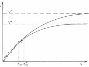
If prediction of responses is recognized as the primary purpose of an investigation then the requirements for the design, execution and analysis of the experiments become different, generally less stringent. This is illustrated (Fig. 7) again on the example of hyperbolic kinetic

experiments described by the Michaelis-Menten equation. If prediction is required only in the low concentration, first-order region (as is frequently the case, for example, in pharmacokinetic applications) then the observations may also be restricted to this range. However, such an experimental design does not permit evaluation of the maximal velocity, V, and therefore the Michaelis-Menten constant, К , can be

estimated also with only great uncertainty. The 2iagram illustrates two pairs of parameters which describe the linear portion equally well. This indicates that one parameter is actually redundant. The linear part of the rate curve can indeed be characterized by a single constant, the ratio of

(27)

V

Fig. 7. Use of unsatisfactorily estimated parameters for prediction.

Response prediction is required only in the approximately linear range of the hyperbola and, therefore, observations are restricted to this range. From these, the maximum velocity (V) and, therefore, the Michaelis constant (1^) can be evaluated only very imprecisely. Consequently, the two pairs of constants,

(V .Kjj ) and (V .Kjn ), are plausible but uncertain estimates.

Still, both pairs provide good prediction in the desired region.

One parameter, V/Km , is sufficient to characterize the rate curve in its linear range, while one constant is redundant.

Consequently, redundant parameters can be applied for response prediction. However, they should not be utilized for mechanistic modelling.

Thus, it is quite appropriate (even if not too elegant) to use a model containing redundant parameters for purposes of prediction. After all, we are not really interested now in the constants or their errors.

They merely serve as a means for the main purpose of the investigation, prediction. This is in sharp contrast with the study of mechanistic

models: We wish to know their parameters with high precision. Consequently, redundant constants will be excluded from deterministic models.

ESTIMATION OF MECHANISTIC MODEL PARAMETERS

As just indicated, evaluation of mechanistic models requires the inclusion of the smallest possible number of interpretable parameters.

This principle of parsimony (Tukey, 1961) means that the mathematical representation of an otherwise plausible model would have to be simplified.

For example, it may not be possible to evaluate some constants of

mechanistically interpretable higher-degree rate equations and, therefore, these may have to be represented by the less complex, more superficial Hill equation (Hurst, 1974; Reich and Zinke, 1974). The situation may arise simply because of the given true magnitude of the natural model constants.

For instance, stepwise equilibrium constants and most cumulative formation constants of the Adair equation, which characterizes most binding systems, cannot be evaluated in the presence of strong positive cooperativities

(Endrényi and Kwong, 1973).

25

(28)

Several methods are frequently available for the assessment of model constants. Again, they include not only statistical but also often very useful graphical procedures. The relative merits of these procedures have been evaluated only in a few instances. For example, various

approaches estimating the two Michaelis-Menten parameters have been compared in computer simulations (Dowd and Riggs, 1965; Colquhoun, 1969;

Endrényi and Kwong, 1972). As illustrated in Table 3 for two specific experimental designs, the precision (reproducibility) and accuracy

(correctness) of parameters obtained by nonlinear regression and from the various linear transformations were noted. Quite consistently, the customarily and still most usually used double reciprocal Lineweaver-Burk plot yielded extremely poor results.

Among the linear plots derived from the hyperbolic expression, the reverse of the Hanes plot, the contrast of c against c/v , gave the best results when the absolute experimental error was constant. This plot excelled also with constant relative errors but only with harmonic and, to some extent, with geometric spacing (Endrényi and Kwong, 1972). The parameters obtained by this linearization have frequently more favourable properties than those based on (weighted) nonlinear regression.

Nevertheless, nonlinear least-squares analysis has advantageous features which recommend its use with asymptotically large samples: The estimated parameters are efficient (have the smallest possible variance), consistent

(essentially, unbiased) and normally distributed (Hartley and Booker, 1965;

Jennrich, 1969; Malinvaud, 1970). For practical purposes it is probably more important that the optimality of these parameter estimates does not deteriorate badly at small sample sizes (Endrényi and Kwong, 1972).

This means also that the parameters obtained by (weighted) nonlinear regression are comparatively robust, that is, while they may not give the best possible results, they will never give very poor, misleading or imprecise answers either. This feature strongly suggests the use of the

(weighted) nonlinear least-squares method.

Some alternative procedures evaluating the Michaelis-Menten parameters have been described recently. They include the separate estimation of the

two parameters on the basis of paired observations (Miguel Merino, 1974;

Fajszi and Endrényi, 1974), and an ingenious graphical procedure determining the constants in parameter space and using nonparametric methods for their assessment (Eisenthal and Cornish-Bowden, 1974).

The evaluation of model constants requires ascertaining not only the • magnitudes of the parameters but also their errors. Unfortunately, this principle is not always followed. At any rate, even the separately expressed parameter errors contain incomplete and somewhat misleading information. For illustration, Fig. 8b shows the separate 99% confidence limits of the two Michaelis-Menten parameters evaluated in an experiment.

Confidence limits estimated jointly for the two constants are also

displayed in the diagram. The separate limits contain an extensive range of parameter combinations which are excluded by the joint limits. On the other hand, some further admissible pairs of constants would not be considered by the separate limits.

The joint limits are slanted upwards thereby indicating that the two parameters are correlated in the positive direction. This is reasonable since together with a larger V value we would expect to determine also a larger value.

(29)

Table 3.

Accuracy and precision of Michaelis-Menten parameters estimated by various methods

Method of estimation

y X

V Mean

G e о m

RMS^(a)b) (c)(d)(e)(f)(g)(h)(i)(j)

e t r i c Кm Mean RMS

A r V Mean

i t h

RMS

m e t i Кm Mean

c

RMS Constant absolute

error

(d) 1/V 1/c 287.1 *(c)

535.0 * 76.8 Л 28.2 *

(e) V v/c 85.2 23.6 71.6 49.3 98.5 20.6 101.3 55.7

(f) c/v c 108.6 28.4 132.3 85.2 108.9 26.9 136.8 95.8

1/c 1/v 101.8 ^* 95.6 * 96.0 * 92.0 *

(g) v/c V 95.6 * 72.3 * 218.0 * 487.1 *

(h) c c/v 96.3 20.0 98.2 60.8 97.0 19.7 97.2 69.7

(i) V c 104.9 23.8 115.6 71.0 107.9 30.2 128.9 108.7

Constant relative error

(d) 1/v 1/c 106.0 * 117.0 * 109.6 * 137.5 *

(e) V v/c 92.7 21.5 85.7 40.9 96.6 20.5 93.8 49.6

(f) c/v c 106.1 22.6 120.0 64.1 103.0 28.3 117.6 98.4

1/c 1/v 139.3 * 177.2 * 97.5 * 95.7 *

(g) v/c V 124.5 299.0 151.5 504.9 126.4 * 171.7 *

(h) c c/v 96.9 17.9 95.6 51.3 88.5 20.4 70.0 71.8

(i) V c 109.4 26.5 124.9 82.8 110.3 37.0 132.6 130.3

(j) v(w) c 103.6 29.3 109.4 58.4 105.9 24.6 117.0 60.4

(a) 750 computer simulated experiments were performed with 5 observations spaced, between relative velocities of 0.20 and 0\80, either in a geometric or in arithmetic progression of concentrations. The true values of the two parameters were assumed to be 100. With constant absolute errors, the standard deviation a = 10, with constant relative errors о^= 0.20v^ .

(b) RMS: Root mean square of the estimated parameter, the square root of the average observed parameter variance.

(c) * indicates RMS > 1000.

(d) Lineweaver, H. and Burk, D. (1934). J. Am. Chem. Soc. 5 6 , 658.

(e) Eadie, G.S. (1942). J. Biol. Chem. 1 4 6 , 85; Hofstee, B.H.J. (1952).

Science 116, 329.

(f) Hanes, C.S. (1932). Biochem. J. 26^ 1406.

(g) Scatchard, G. (1949). Ann. N.Y. Acad. Sei. 51, 660.

(h) Endrényi and Kwong (1972).

(i) Nonlinear regression.

(j) Weighted nonlinear regression.

27

(30)

Fig. 8. Separate and joint parameter confidence limits.

Approximate 90 and 99% confidence limits (a=0.10 and 0.01, respectively) to a given set of hyperbolic kinetic observations based (a) on elliptical contours (linear approximation), and

(b) on sum-of-squares contours. The latter are nearly elliptical.

The second diagram includes also the 99% limits estimated

separately for the two parameters. They include a large range of parameter pairs which is excluded by the joint limits.

(c) The approximately elliptical shape of the sum-of-squares contours is distorted further away from the minimum which is indicated by a + sign. (d) Contours in the inadmissible region of negative К values,

m

The joint confidence limits actually represent a given, constant value of the sum of squares. Consequently, as comparison of Figs. 8b and 8c indicates, the elliptical shape of the sum-of-squares contours (projected sections of the sum-of-squares surface) are gradually distorted with in

creasing distance from the minimum. This can be seen further in Fig. 8d which shows contours at negative К values.

In spite of their usefulness, confidence and sum-of-squares contours have scarcely been applied until now.

(31)

SUMMARY

1. An investigator must know very clearly the primary purpose of his/her investigation. In particular, it should be realized whether the observations aim mainly at the future prediction 'of the responses

(empirical models) or at gaining insight into natural phenomena, including mechanisms of processes (mechanistic or deterministic models).

2. The effective design and analysis of experiments depend on their purposes: (a) prediction, (b) identification of mechanistic models, or

(c) evaluation of their parameters. Response prediction does not necessarily require precisely estimated parameters and it may rely on redundant constants.

3. Features and procedures of model building are illustrated on the example of the hyperbolic Michaelis-Menten equation which characterizes the Briggs-Haldane mechanism of simple enzymic reactions.

4. Designing the experiments in accordance with their primary purpose assists their evaluation and can substantially improve the reliability of the conclusions. For instance, provided that the absolute observational error tends to remain constant throughout the range of experimentation, the precision and accuracy of the estimated Michaelis-Menten equation improve by restricting the range of observations to relative velocities exceeding at least the 0.2.

5. Analysis by the method of least squares requires that the error behaviour (for instance, constant absolute or constant relative error) be known or at least assumed. The experimental design and the conclusions reached by the analysis can be vastly different depending on the actual and assumed error structure. Assumptions about the distribution of errors are required only for the calculation of confidence limits and statistical significance tests.

6. Residual plots are very useful for testing the validity of an assumed model and for evaluating the error behaviour.

7. Especially in more complex systems, graphical and statistical procedures frequently supplement each other. Each method has its

limitations. Therefore, conclusions concerning model validity and parameter values should be reached by the joint application of several procedures.

ACKNOWLEDGEMENT

This work was supported by the Medical Research Council of Canada.

REFERENCES

Ainsworth, S. (1968). J. Theor. Biol. 19^, 1.

Atkins, G.L. (1971). Biochim. Biophys. Acta 252, 405.

Augustinsson, K.B., Bartfai, T. and Mannervik, B. (1974). Biochem. J.

141, 825.

Bartfai, T., Ekwall, K. and Mannervik, B. (1973). Biochemistry 12, 387.

Bartfai, T. and Mannervik, B. (1972). FEBS Letters 2 6 , 252.

Bliss, C.I. and James, A.T. (1966). Biometrics 2 2 , 573.

Box, G.E.P. and Cox, D.R. (1964). J. Roy. Stat. Soc. B 2 6 , 211.

Box, G.E.P. and Hill, W.J. (1967). Technometrics £, 57.

Box, G.E.P. and Hill, W.J. (1974). Technometrics 1 6 , 385.

Box, G.E.P. and Hunter, W.G. (1962). Technometrics U_, 301.

Box, G.E.P. and Jenkins, G.M. (1970). in "Time Series Analysis, Forecasting and Control" (Holden-Day, San Francisco), pp. 248-250.

Box, G.E.P. and Lucas, H.L. (1959). Biometrika 46^, 77.

29

(32)

Cleland, W.W. (1963). Nature 198, 463.

Cleland, W.W. (1967). Adv. Enzymol. 29,1.

Colquhoun, D. (1969). Appl. Statist. 1 8 , 130.

Cornish-Bowden, A. and Koshland, D.E., Jr. (1970). Biochemistry 9^, 3325.

Daniel, C. and Wood, F.S. (1971). in "Fitting Equations to Data"

(Wiley-Interscience, New York) pp. 28-29, 34-43.

Dowd, J.E. and Riggs, D.S. (1965). J. Biol. Chem. 2 4 0 , 863.

Draper, N.R. and Smith, H. (1966). in "Applied Regression Analysis"

(Wiley, New York), pp. 86-93.

Eisenthal, R. and Cornish-Bowden, A. (1974). Biochem. J. 1 3 9 , 715.

Endrényi, L., Chan, M.S. and Wong, J.T.F. (1971). Can. J. Biochem.

49, 581.

Endrényi, L. and Kwong, F.H.F. (1972). in "Analysis and Simulation of Biochemical Systems", eds. H.C. Hemker and B. Hess (North-Holland, Amsterdam), p. 219.

Endrényi, L. and Kwong, F.H.F. (1973). Acta Biol. Med. Germ. 31, 495.

Fajszi, Cs. and Endrényi, L. (1974). FEBS Letters 4 4 , 240.

Glejser, H. (1969). J. Am. Stat. Assoc. 6 4 , 316.

Goldfeld, S.M. and Quandt, R.E. (1965). J. Am. Stat. Assoc. 6 0 , 539.

Hartley, H.O. and Booker, A. (1965). Ann. Math. Stat. 3 6 , 638.

Hunter, W.G., Hill, W.J. and Wiehern, D.W. (1968). Technometrics 10, 145.

Hurst, R.O. (1974). Can. J. Biochem. 5 2 , 1137.

Jennrich, A.I. (1969). Ann. Math. Stat. 4 0 , 633.

Kendall, M.G. and Stuart, A. (1966). in "The Advanced Theory of Statistics"

(Hafner, New York), Vol. 3, pp. 361-362, 403-404.

Kwong, F.H.F. (1972). M.Sc. Thesis, University of Toronto, pp. 73-90.

Malinvaud, E. (1970). Ann. Math. Stat. 4 1 , 956.

Miguel Merino, F. (1974). Biochem. J. 143, 93.

Moosavi, S.F.H. and Endrényi, L. (1974). Proc. Can. Fed. Biol. Soc.

17, 162.

Ottaway, J.H. (1973). Biochem. J. 134, 729.

Pettersson, G. and Pettersson, I. (1970). Acta Chem. Scand. 2_4, 1275.

Reich, J.G. (1974). Studia Biophys. 42, 165.

Reich, J.G., Wangermann, G., Falck, M. and Rohde, K. (1972). Eur. J.

Biochem. 2 6 , 368.

Reich, J.G. and Zinke, I. (1974). Studia Biophys. 4 3 , 91.

Suranyi, G. (1973). M.Sc. Thesis, University of Toronto, pp. 45-53.

Tukey, J.W. (1961). Technometrics 3,, 191.

Wilkinson, G.N. (1961). Biochem. J. 8 0 , 324.

(33)

Sym p. Biol. Hung. 18, pp. 31-46 (1974)

R E G U L A T O R Y P R O P E R T I E S O F D I S S O C I A T I N G A N D A S S O C I A T I N G E N Z Y M E S Y S T E M S

B . I . K u r g a n o v

I n s t i t u t e f o r V i t a m i n R e s e a r c h , M o s c o w , U S S R

I N T R O D U C T I O N

A l l a l l o s t e r i c e n z y m e s p o s s e s s a s u b u n i t s t r u c t u r e . A t c e r  t a i n c o n d i t i o n s t h e y r e v e a l t h e p o s s i b i l i t y t o d i s s o c i a t e i n t o i n d i v i d u a l s u b u n i t s w h i c h a r e u s u a l l y e n z y m a t i c a l l y i n a c t i v e . O n t h e o t h e r h a n d , t h e m o l e c u l e s o f a l l o s t e r i c e n z y m e s o f t e n c o n t a i n t h e a d d i t i o n a l a s s o c i a t i o n s i t e s w h o s e s a t u r a t i o n o c c u r s a t a s s o c i a t i o n o f p r o t e i n m o l e c u l e s . T h e t y p i c a l s i t u a t i o n i s t h a t t h e s i m i l a r a s s o c i a t i o n i s a c c o m  p a n i e d b y d i m i n u t i o n o f s p e c i f i c e n z y m e a c t i v i t y o w i n g t o

s t e r i c s c r e e n i n g o f a c t i v e s i t e s .

T h e d i s p l a c e m e n t o f e q u i l i b r i u m b e t w e e n o l i g o m e r i c e n z y  m e f o r m s u n d e r t h e i n f l u e n c e o f m e t a b o l i t e s i s o n e o f t h e a l l o s t e r i c m e c h a n i s m s o f e n z y m e r e g u l a t i o n i n v i v o ( D a t t a e t a l . ,196^-; K u r g a n o v ,1 9 6 7, 1 9 6 8 ; N i c h o l e t a l . , 1 9 6 ? ; F r i e d e n , 1 9 6 7,1 9 6 8; B o n s i g n o r e e t a l . ,1 9 6 8; L e J o h n e t a l . ,1 9 6 9; C o n - s t a n t i n i d e s a n d D e a l , 1 9 ^ 9 ; S t a n c e l a n d D e a l , 1 9 6 9 ) « I t i s w o r t h n o t i n g t h a t t h e r e g u l a t o r y c h a r a c t e r i s t i c s o f p o l y m e  r i s i n g a l l o s t e r i c e n z y m e s y s t e m s ( t h e s h a p e o f t h e d e p e n d e n  c e s o f e n z y m a t i c r e a c t i o n r a t e o n c o n c e n t r a t i o n o f s u b s t r a t e

31

(34)

o r a l l o s t e r i c e f f e c t o r , t h e c h a r a c t e r o f c o m b i n e d a c t i o n o f a l l o s t e r i c l i g a n d s o n e n z y m a t i c ' a c t i v i t y a n d s o o n ) d e p e n d s o n e n z y m e c o n c e n t r a t i o n .

T h e k i n e t i c a p p r o a c h e s t o a n a l y s i s o f k i n e t i c b e h a v i o u r o f d i s s o c i a t i n g a n d a s s o c i a t i n g a l l o s t e r i c e n z y m e s y s t e m s w e r e e l a b o r a t e d b y K u r g a n o v ( 1 9 6 7 , 1 9 6 8 ) . T h e s e a p p r o a c h e s a l l o w t o p r o v e t h e e x i s t e n c e o f a l l o s t e r i c i n t e r a c t i o n s m e d i  a t e d b y t h e d i s p l a c e m e n t o f e q u i l i b r i u m b e t w e e n o l i g o m e r i c e n z y m e f o r m s u n d e r t h e i n f l u e n c e o f s u b s t r a t e s a n d a l l o s t e r i c e f f e c t o r s a n d i s o l a t e a l l o s t e r i c i n t e r a c t i o n s i n i n d i v i d u a l o l i g o m e r i c f o r m s . T h e s e p a r a t i o n o f s u c h t w o t y p e s o f a l l o s  t e r i c i n t e r a c t i o n s b e c o m e s p o s s i b l e i f o n e a n a l y s e s t h e s e t o f t h e d e p e n d e n c e s o f s p e c i f i c e n z y m e a c t i v i t y o n e n z y m e c o n  c e n t r a t i o n s o b t a i n e d a t v a r i o u s f i x e d c o n c e n t r a t i o n s o f s u b  s t r a t e a n d a l l o s t e r i c e f f e c t o r s .

T a k i n g i n t o a c c o u n t t h e g r e a t i m p o r t a n c e o f t h e d e p e n d e n  c e s o f s p e c i f i c e n z y m e a c t i v i t y ( i . e . i n i t i a l v e l o c i t y o f e n z y m a t i c r e a c t i o n d i v i d e d b y e n z y m e c o n c e n t r a t i o n ) o n c o n  c e n t r a t i o n o f e n z y m e a t a n a l y s i s o f k i n e t i c b e h a v i o u r o f d i s s o c i a t i n g a n d a s s o c i a t i n g a l l o s t e r i c e n z y m e s y s t e m s , I d e c i d e d t o d e v o t e m y r e p o r t t o t h e d i s c u s s i o n o f t h e c h a r a c  t e r o f s p e c i f i c e n z y m e a c t i v i t y v e r s u s e n z y m e c o n c e n t r a t i o n p l o t s f o r p o l y m e r i s i n g e n z y m e s y s t e m s o f d i f f e r e n t t y p e s .

A S S O C I A T I N G E N Z Y M E S Y S T E M S O F T H E T Y P E M O N O M E R 5 = ± N - M E R

T h e d e p e n d e n c e o f s p e c i f i c e n z y m e a c t i v i t y o n e n z y m e c o n c e n  t r a t i o n i s d e t e r m i n e d b y t h r e e p a r a m e t e r s f o r t h e a s s o c i a  t i n g e n z y m e s y s t e m s o f t h e t y p e m o n o m e r N - m e r . T h e s e