Szakaszos gyártócella szimulációja és irányítása

(1)

DOKTORI (PhD) ÉRTEKEZÉS

BALATON MIKLÓS GÁBOR

Pannon Egyetem 2014.

DOI: 10.18136/PE.2014.561

(2)

(3)

Pannon Egyetem

Vegyészmérnöki és Folyamatmérnöki Intézet Folyamatmérnöki Intézeti Tanszék

Szakaszos gyártócella szimulációja és irányítása

DOKTORI (PhD) ÉRTEKEZÉS

Balaton Miklós Gábor

Konzulensek

Dr. Nagy Lajos, egyetemi docens Dr. Szeifert Ferenc, egyetemi docens

Vegyészmérnöki- és Anyagtudományok Doktori Iskola Pannon Egyetem

2014.

(4)

University of Pannonia

Institute of Chemical and Process Engineering Institutional Department of Process Engineering

Simulation and control of batch processing units

PhD Thesis

Miklós Gábor Balaton

Supervisors

Lajos Nagy PhD, associate professor Ferenc Szeifert PhD, associate professor

Doctoral School in Chemical Engineering and Material Sciences University of Pannonia

2014.

(5)

SZAKASZOS GYÁRTÓCELLA SZIMULÁCIÓJA ÉS IRÁNYÍTÁSA Értekezés doktori (PhD) fokozat elnyerése érdekében a

Pannon Egyetem Vegyészmérnöki- és Anyagtudományok Doktori Iskolájához tartozóan.

Írta:

Balaton Miklós Gábor Témavezetők: Dr. Nagy Lajos

Elfogadásra javaslom (igen / nem) ……….

(aláírás) Dr. Szeifert Ferenc

Elfogadásra javaslom (igen / nem) ……….

(aláírás) A jelölt a doktori szigorlaton ...%-ot ért el,

Az értekezést bírálóként elfogadásra javaslom:

Bíráló neve: …... …... igen /nem

……….

(aláírás) Bíráló neve: …... …...) igen /nem

……….

(aláírás)

A jelölt az értekezés nyilvános vitáján …...%-ot ért el.

Veszprém, ……….

a Bíráló Bizottság elnöke A doktori (PhD) oklevél minősítése…...

………

Az EDHT elnöke

(6)

Köszönetnyilvánítás

Köszönetet mondani mindig egy felemelő érzés, mivel mindig valami lezárásaként tesszük, ami egyben egy új dolog kezdetét is jelenti. Nagy viszontagságok között készült el ez a dolgozat, többször is elbizonytalanodtam, hogy egyáltalán be tudom-e fejezni. Nagy áldozatokat kellett hoznom azért, hogy eljuthassak a köszönetnyilvánítás megírásáig, azaz a dolgozat befejezéséig. De végül sikerült.

Elsősorban témavezetőimnek Dr. Nagy Lajosnak és Dr. Szeifert Ferencnek szeretném megköszönni a rengeteg segítséget és szakmai útmutatást, amit kaptam tőlük az évek során. Valamint szeretném megköszönni a tanszéki kollektívának a számos építő jellegű szakmai vitát, amelyek nélkül nem tudtam volna ennyit fejlődni. A PhD-s csapatnak (Rádi György, Szabó László, Dobos László, Tóth Richárd, Egedy Attila, Bárkányi Ágnes, Borsos Ákos, Király András) is szeretném megköszönni a számos közös utazást és élményt, ami a PhD-s évek alatt megéltünk együtt.

Szeretném még megköszönni családomnak is az egyetemi éveim alatti támogatást, ami nélkül nem készült volna el ez a dolgozat sem.

Nagyon sok köszönettel tartozom minden barátomnak, ismerősömnek, aki tartotta bennem az erőt a nehéz időkben is, és bíztatott a dolgozat befejezésére.

(7)

Kivonat

A gyógyszer-, élelmiszer-, polimer- és finomvegyszer iparban a szakaszos (rugalmas) technológiai rendszerek gyakori eleme a keverővel ellátott fűthető- hűthető autokláv, amelyben a reagáltatáson túlmenően számos más művelet (desztilláció, extrakció, kristályosítás, stb.) is elvégezhető. Szakaszos reaktorok esetén a legfontosabb szabályozott jellemző a hőmérséklet, mivel a magas hozzáadott értékű termékek előállítása során a hőmérséklet elégtelen szabályozása esetén nem megfelelő termék keletkezhet, amely jelentős anyagi veszteséget okozhat, illetve a gyógyszeriparban felhasználhatatlan komponenst eredményezhet. Miközben az irányítási rendszer gyakorlati megvalósítását jól segíti az S88 szabvány, a különböző szintű irányítási algoritmusok kialakítását számos elméleti és gépészeti probléma nehezíti. A kutatás elsősorban a magasabb hierarchia szintek összetettebb irányítási problémáira irányul mint például az optimalizálás, ütemezés, stb. Ugyanakkor, az alacsonyabb szintek megoldatlan irányítástechnikai problémái a felsőbb hierarchia szintű megoldások realizálását lehetetlenné teszik.

Vegyipari gyártó rendszerek gépészeti tervezését és kivitelezését, különösen a mérőműszerek elhelyezését és beépítését gyakran a praktikusság és az esztétikai elvek vezérlik. Klasszikus szabályozó algoritmusok esetén (PID szabályozó) ezek a hibák viszonylag ritkán okozzák a szabályozás elégtelenségét, viszont magasabb szintű illetve modell alapú szabályozási algoritmusok esetén jelentős akadályokat jelenthetnek. A mérőműszerek és technológiai rendszer részletes vizsgálata és beállítása nélkül magasabb szintű irányítási algoritmusokkal nem érhető el jobb minőségű szabályozás (vagy csak rosszabb) a klasszikus megoldásokhoz képest.

Az iparban egyre inkább terjednek a három hőmérsékleti szinttel rendelkező hűtő-fűtő rendszerek, amelyek alkalmazása energiafelhasználás szempontból előnyös, viszont a köpeny hőmérsékletszabályozását bonyolultabbá teszik. A középső hőmérsékleti szint mind hűtő mind fűtő szerepet is betölthet a reaktor állapotától függően. A klasszikus két üzemmódot kezelő split-range megoldások nem alkalmasak ezen rendszer kezelésére, ezért új megoldás kidolgozására volt szükség.

Olyan split-range algoritmusok kerültek kidolgozásra, amelyek a klasszikus hőmérsékletszabályozási megoldásokhoz (PID) kapcsolhatóak. Az első split-range algoritmus során a köpeny és a belépő közeg hőmérsékletét figyelembe véve, valamint a köpeny recirkulációt mint keverő modellt felhasználva, a szabályozó különböző előre definiált karakterisztikák között vált, amivel elérhető, hogy a szabályozott objektum erősítésének előjele ne változzon. Ezzel megvalósítható, hogy mindhárom közeget megfelelően tudja kihasználni a köpenyhőmérséklet szabályozó.

A kutatás során egy második split-range algoritmus kifejlesztésére is sor került. A szerző különböző köpenymodellek felhasználásával két modell alapú split-range megoldást is kidolgozott. Mindkét megoldás esetén nemcsak a szabályozott objektum erősítésének előjele, hanem annak értéke is változatlanul tartható. A különböző split-range algoritmusok vizsgálata nem csak MATLAB környezetben végzett szimulációval történt, hanem a tanszéki laboratóriumban található félüzemi szakaszos gyártócellán végzett mérésekkel is.

(8)

Abstract

The heatable, coolable, and stirred autoclaves are common parts of batch technologies in the pharmaceutical-, food-, polymer- and fine-chemical industries.

Beyond performing chemical reactions also several other operations can be performed in autoclaves as well (distillation, extraction, crystallization, etc.). In the case of batch reactors, the most important controlled variable is temperature, since in the manufacturing processes of high-value-added products, insufficient control might produce off-grade product that can cause significant financial loss, and in the pharmaceutical industry result in an unusable batch. While the practical implementation of the control system is supported by the S88 standard, the implementation of control algorithms at different hierarchy levels are encumbered by theoretical and mechanical problems. The scientific research mainly focuses on the more complex problems of the higher hierarchy levels, e.g., optimization, scheduling, etc. However, the unsolved control problems of the lower hierarchy levels make the realization of the higher hierarchy solutions impossible.

In the mechanical design and construction of chemical manufacturing systems, especially the location and implementation of measuring instruments are commonly driven by aesthetic and practical principles. When using classical control solutions (e.g., Proportional Integral Derivative (PID) controller), these errors rarely cause poor control performance; however, in the case of advanced and model-based control algorithms the control performance is significantly affected. Without the detailed analysis and tuning of the measuring instruments and the technology itself, better control performance cannot be achieved (or even worse) compared to classical control solutions.

In the industry an increasing number of heating/cooling systems utilizing three different temperature levels can be found, which are advantageous from an economic point of view; however, it makes the control more complicated. The medium temperature level can also be a heating or cooling media depending on the actual state of the reactor. The classical split-range solution handling two modes of operation are not suitable for such systems, thus the development of new solutions is needed.

Such split-range algorithms were developed that can be used together with classical control solutions (PID). The first split-range algorithm considers the actual temperature value of the jacket and the inlet thermal fluid. According to the mixer-based model describing the jacket recirculation loop, it switches between a set of predefined splitting characteristics with the aim to avoid the change in the sign of the gain of the controlled object. With this solution the adequate utilization of all three temperature levels by the jacket-temperature controller can be achieved.

A second split-range algorithm was also developed. To describe the jacket recirculation loop two modelling considerations were used. In both solutions not only the sign of the gain of the controlled object, but also the value of the gain is kept unchanged. The testing and analysis of the different split-range solutions were not only performed by MATLAB based simulation but also by test measurements on the pilot batch processing system, located in the laboratory of

(9)

Auszug

Die beheizbare, kühlbare, mit einem Mixer ausgestattete Autoklaven sind häufig Bestandteil von Batch-Technologien in der Pharma-, Lebensmittel-, Poly- mer- und Feinchemie Industrie, in der zusätzlich zur Reaktion eine Anzahl von anderen Operationen (Destillation, Extraktion, Kristallisation, usw.) durchgeführt werden kann. Im Falle von Batch-Reaktoren der wichtigste Regelparameter ist die Reaktionstemperatur, weil die unzureichende Temperaturregelung in der Produk- tion vom Hochwertprodukten zu nicht-konformen Produkte führen kann, die Folge können erheblichen finanziellen Verlusten als auch Entstehung von nutzlo- sen Komponenten in der Pharmaindustrie sein. Während die praktische Imple- mentierung des Produktionskontrollsystems vom S88-Standard unterstützt wird die Entwicklung von Regelalgorithmen wird von einen Reihe von theoretischen und mechanischen Problemen erschwert. Die Forschung konzentriert sich vor allem auf komplex Kontrollprobleme von höheren hierarchischen Ebenen wie Optimierung, Planung, usw., jedoch die ungelösten Probleme auf unteren Ebenen machen es unmöglich die höheren hierarchieebenen Lösungen zu realisieren.

Die mechanische Planung und Konstruktion von Produktionssystemen der chemischen Industrie insbesondere die Platzierung und Installation der Messin- strumente werden oft von Praktischer Anwendbarkeit und ästhetischen Prinzipien angetrieben. Im Falle der klassischen Regelalgorithmen (PID) diese Fehler verur- sachen nur selten unzureichende Regelung, jedoch sie können erhebliche Hinder- nisse bei übergeordneten und modellbasierten Regelalgorithmen darstellen. Im Vergleich zur klassischen Lösungen ohne eingehende Prüfung und Einstellung der Messinstrumente und Technology mit übergeordneten Regelalgorithmen kann keine bessere (oder noch schlimmer) Regelung erreicht werden.

Kühl-und Heizsysteme mit drei Temperaturstufen werden sich immer mehr in der Industrie verbreiten, was in Hinblick auf den Energieverbrauch vorteilhaft ist, jedoch die Manteltemperaturregelung kompliziert. Die mittlere Temperatur Ebene kann je nach dem Status des Reaktors sowohl Heiz- als auch Kühlmedien sein. Dieses System kann von klassischen zwei-mode Split-Range Lösungen nicht behandelt werden, deshalb war es notwendig neue Lösungen zu entwickeln.

Solche Split-Range Algorithmen wurden entwickelt, die mit den klassischen Temperaturregelung-Lösungen (PID) zu gleicher Zeit verwendbar sind. Es wird im ersten Split-Range Algorithmus unter Berücksichtigung der Mantel- und Zulauftemperatur sowie unter Einsatz vom Mantel Rezirkulation als Mischmodell zwischen verschiedene vordefinierte Regelcharakteristik umgeschaltet, um zu vermeiden, dass das Vorzeichen der Verstärkung des geregelten Objekts sich ändert. Mit dieser Lösung kann die angemessene Nutzung aller drei Temperaturen Ebene vom Manteltemperaturregler erreicht werden.

Während der Forschung wurde auch ein zweiter Split-Range Algorithmus entwickelt. Um die Mantel Rezirkulierungsschleife zu beschreiben zwei modellbasierte Split-Range Lösungen wurden ausgearbeitet. In beiden Lösungen wird nicht nur das Vorzeichen der Verstärkung des geregelten Objekts sondern auch ihr Zeitwert unverändert beibehalten. Der Test der verschiedenen Split- Range-Algorithmen wurde nicht nur in MATLAB simuliert sondern auch mit Messungen auf der Pilot Serienproduktion-Zelle im Lehrstuhllabor durchgeführt.

(10)

List of Figures

Figure 1.1: Direct heating/cooling without recirculation ... 5

Figure 1.2: Direct heating and direct cooling jacket configuration ... 6

Figure 1.3: Indirect heating and direct cooling jacket configuration ... 7

Figure 1.4: Indirect heating and indirect cooling jacket configuration ... 7

Figure 1.5: Monofluid heating/cooling jacket configuration ... 9

Figure 1.6. Cascade control of the reactor temperature... 14

Figure 1.7. The temperature control configuration of the batch reactor ... 15

Figure 1.8. Split-range algorithm for two modes of operation ... 16

Figure 2.1. Flowsheet of the batch processing unit ... 20

Figure 2.2. The temperature dependence of the thermal fluid ... 20

Figure 2.3: The monofluid thermoblock ... 21

Figure 2.4: The control logic of the electric heaters ... 22

Figure 2.5: The batch reactor, feeding and weighing tanks, vapour product condenser, and product collectors... 23

Figure 2.6: The control scheme of the batch processing unit (before 2010) ... 24

Figure 2.7: The control scheme of the batch processing unit (after 2010) ... 25

Figure 2.8: Flowsheet of the pilot-plant-size batch processing unit, – the original configuration (2007-2009) ... 26

Figure 2.9 Flowsheet of the pilot-plant-size batch processing unit, – after the first modification (2009-2010) ... 27

Figure 2.10: Flowsheet of the pilot-plant-size batch processing unit, – after the final modification (2010-present day)... 28

Figure 2.11. Different thermometer installations in a pipe bend... 29

Figure 2.12: The change of the direction in the case of the jacket inlet and outlet thermometers ... 30

Figure 2.13. The effect of the incorrect installation of the jacket inlet and outlet thermometers ... 30

Figure 2.14: The temperature measuring chain ... 31

Figure 2.15: Test configuration for comparing the dynamics of the different thermometers ... 32

Figure 2.16: The tested thermometers ... 33

Figure 2.17: The difference in dynamic behaviour of the tested thermometers ... 34

Figure 2.18: The test measurements to identify the relative offsets, time constants, and dead times of the thermometers ... 35

Figure 2.19: The dynamic behaviour of the final thermometers ... 35

Figure 2.20: The temperature-dependent offset compared to the jacket outlet thermometer ... 36

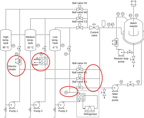
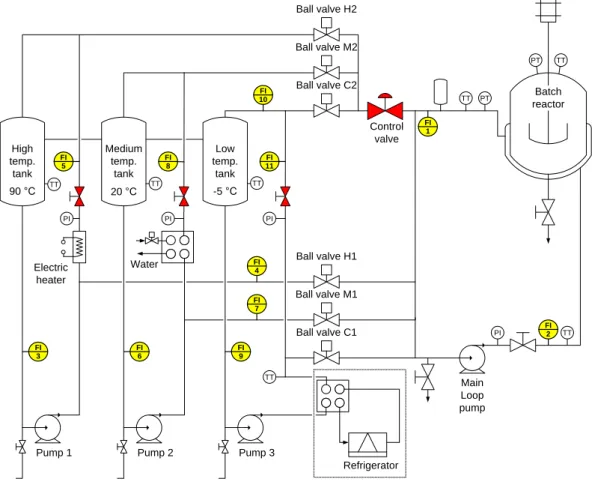
Figure 2.21: The measuring points and valves used for recording the hydrostatic characteristics of the system... 37

Figure 2.22: The FLEXIM FLUXUS F601 ultrasonic flow meter ... 38

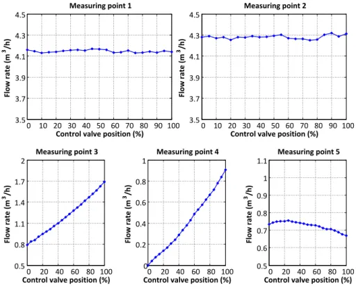
Figure 2.23: The hydrostatic characteristics in measuring point 3 – 5 ... 40

(12)

Figure 2.24: Hydrostatic characteristics at the tuned operating point for the high-

temperature loop ... 41

Figure 2.25: Hydrostatic characteristics at the tuned operating point for the medium- temperature loop ... 42

Figure 2.26: Hydrostatic characteristics at the tuned operating point for the low- temperature loop ... 42

Figure 2.27: Flowsheet of the reaction heat physical simulation loop ... 43

Figure 2.28: The expected and calculated (from raw data) heat flow characteristics of the electric heater ... 45

Figure 2.29: Measurement for identifying the parameters of the temperature-dependent offset and the first-order exponential filter ... 45

Figure 2.30: The modules for compensating the measured raw temperature signal of the thermometer after the heater ... 46

Figure 2.31: The temperature-dependent offset between the T_reactor and T_after_heater ... 47

Figure 2.32: Measurement for recording the output heat flow of the electric heater ... 47

Figure 2.33: The heat flow characteristics of the electric heater calculated from both the raw and filtered data ... 48

Figure 3.1: The logo of the batch reactor thermal parameter identifying application ... 51

Figure 3.2: The batch reactor configuration feasible for BRIEW ... 52

Figure 3.3: The worksheet for composing the required data ... 53

Figure 3.4: The worksheet for choosing the desired equations, limits of the parameters, and the conditions of the used measurement ... 54

Figure 3.5: The flowsheet of the thermal parameter identification... 55

Figure 3.6: The worksheet showing the results of the identification with temperature dependency only ... 56

Figure 3.7: The worksheet showing the results of the identification with temperature and agitator speed dependency ... 56

Figure 3.8: The worksheet for the simulation results ... 57

Figure 3.9: The worksheet for calculating PID parameters ... 58

Figure 3.10: Pop-up window for choosing optional functions ... 59

Figure 3.11: The flowsheet of the reactor heating-up simulation ... 59

Figure 3.12: The worksheet for the heating-up simulation of the reactor ... 59

Figure 3.13: The calculation process of the reaction heat flow ... 61

Figure 3.14: The flowsheet of the reaction heat calculation ... 61

Figure 3.15: Resulting diagram of the reaction heat flow calculation ... 62

Figure 3.16. First step of building the process model ... 64

Figure 3.17. Second step of building the process model ... 65

Figure 3.18. Location of measurements (blue) and parameters to be identified (red) in the case of the hydrodynamic parameter identification of the high-temperature loop ... 66

Figure 3.19. Location of measurements (blue) and parameters to be identified (red) in the case of the hydrodynamic parameter identification of the jacket recirculation loop ... 66

Figure 3.20. Third step of building the process model ... 68

Figure 3.21. Location of measurements (blue) and parameters to be identified (red) in the case of the thermal parameter identification of the high- and low-temperature loop .... 69

(13)

Figure 3.22. Measurement and simulation results for the identification of the thermal parameters of the (a) high- and (b) medium-temperature monofluid thermoblock loops

... 70

Figure 3.23. Measurement and simulation results for the identification of the thermal parameters of the low-temperature monofluid thermoblock loop ... 70

Figure 3.24. Location of measurements (blue) and parameters to be identified (red) in the case of the thermal parameter identification of the jacket recirculation loop and the batch reactor ... 71

Figure 3.25. Measurement and simulation results (first modelling solution, constant heat transfer coefficient, high and medium temperature levels) ... 72

Figure 3.26. Measurement and simulation results using the thermometer models ... 73

Figure 3.27. Temperature dependency of dynamic viscosity in the case of the water and ethylene glycol mixture ... 73

Figure 3.28. Measurement and simulation results (first modelling solution, detailed heat transfer coefficient calculation, high and medium temperature levels) ... 74

Figure 3.29. Measurement and simulation results (first modelling solution, detailed heat transfer coefficient calculation, high and low temperature levels) ... 75

Figure 3.30. Schematic structure of the separator with tube bundle in UniSim Design ... 76

Figure 3.31. Measurement and simulation results (separator with a tube bundle, constant heat transfer coefficient, high- and medium temperature levels) ... 76

Figure 4.1. The structure of the constrained PI controller ... 78

Figure 4.2. The splitter block in case of reactor temperature control ... 78

Figure 4.3. The structure of the jacket recirculation loop ... 79

Figure 4.4. The gain of the slave loop object in the case of the mixer model ... 81

Figure 4.5. The resulting split-range characteristics in the case of the first, mixer model- based split-range algorithm ... 82

Figure 4.6. The gain of the controlled composite object in the case of the first, mixer model-based split-range algorithm ... 82

Figure 4.7. The gain of the controlled object in the slave loop containing only the third split-range characteristic ... 83

Figure 4.8. Example of split-range characteristics at different jacket temperature values for the second, mixer model-based split-range algorithm ... 85

Figure 4.9. The gain of the controlled composite object in the case of the second, mixer model-based split-range algorithm ... 85

Figure 4.10. The gain of the slave loop object in the case of the jacket recirculation loop model ... 87

Figure 4.11. Example of split-range characteristics at different jacket temperature values for the jacket recirculation loop model-based split-range algorithm ... 89

Figure 4.12. The gain of the controlled composite object in the case of the jacket recirculation loop model-based split-range algorithm ... 89

Figure 4.13: The structure of the MATLAB Simulink model for the simulation tests ... 91

Figure 4.14: Split-range characteristic used in the industry... 93

Figure 4.15: Simulation results of the slave control loop in the case of the industrial split- range solution (without reaction heat flow) ... 93

Figure 4.16. Simulation results of the slave control loop in the case of the first split-range algorithm based on the mixer model (without reaction heat flow) ... 94

(14)

Figure 4.17. Simulation results of the slave control loop in the case of the first split-range algorithm based on the mixer model (with reaction heat flow) ... 95 Figure 4.18. Simulation results of the slave control loop in the case of the second split- range algorithm based on the mixer model (without reaction heat flow) ... 96 Figure 4.19. Simulation results of the slave control loop in the case of the second split- range algorithm based on the mixer model (with reaction heat flow) ... 96 Figure 4.20. Simulation results of the slave control loop in the case of the split-range algorithm based on the jacket recirculation loop model (without reaction heat flow) .... 97 Figure 4.21. Simulation results of the slave control loop in the case of the split-range algorithm based on the jacket recirculation loop model (with reaction heat flow) ... 97 Figure 4.22: The structure of the MATLAB Simulink model for the test measurements . 101 Figure 4.23. Test measurement results of the slave control loop in the case of the first split-range algorithm based on the mixer model (without reaction heat flow) ... 102 Figure 4.24. Test measurement results of the slave control loop in the case of the first split-range algorithm based on the mixer model (with reaction heat flow) ... 103 Figure 4.25. Test measurement results of the slave control loop in the case of the second split-range algorithm based on the mixer model (without reaction heat flow) ... 104 Figure 4.26. Test measurement results of the slave control loop in the case of the second split-range algorithm based on the mixer model (with reaction heat flow) ... 104 Figure 4.27. Test measurement results of the slave control loop in the case of the split- range algorithm based on the jacket recirculation loop model (without reaction heat flow) ... 105

(15)

List of Tables

Table 2.1. Details of the jacket thermometers ... 34

Table 2.2. The time constant and dead time values of the final thermometers ... 35

Table 2.3. The parameters to calculate the temperature-dependent offset ... 36

Table 2.4. The number of turns to fully open and the number of measuring positions in the case of the throttle valves ... 39

Table 2.5: The parameters of the temperature-dependent offset ... 46

Table 3.1. Measured values used for the identification of hydrodynamic parameters of the high-temperature loop ... 67

Table 3.2. Identified thermal parameters of the monofluid thermoblock loops ... 69

Table 4.1. Ordering the possible steady-state temperatures in different cases in the algorithm based on the mixer model ... 84

Table 4.2. Choosing the adequate mode of operation ... 84

Table 4.3. Ordering the possible steady-state temperatures in different cases in the algorithm based on the jacket recirculation loop model ... 88

Table 4.4: The conditions for the different simulation tests performed ... 92

Table 4.5: The summary of the different simulation tests performed ... 98

Table 4.6: Utility prices ... 99

Table 4.7: The calculation of the prices of the different temperature levels ... 100

Table 4.8: The utility cost of the different simulation tests ... 100

Table 4.9: The summary of the different test measurements performed ... 101

Table 4.10: The utility cost of the different test measurements ... 106

(16)

Abbreviations

AD Analogue digital

APC Advanced Process Control

BFGS Broyden–Fletcher–Goldfarb–Shanno

BRIEW Batch Reactor Identification Excel Workbook CAPD Computer-Aided process design

CAPE Computer-aided process engineering

CMA-ES Covariant Matrix Adaptation Evolutionary Strategy CSTR Continuously Stirred Tank Reactor

DCS Distributed Control System DP Decentralized Peripherals EA Evolutionary Algorithm HMI Human Machine Interface HTL High Temperature Level

ID Inner Diameter

IP Internet Protocol

LTL Low Temperature Level

MIMO Multiple Input, Multiple Output MPC Model Predictive Controller

MS Microsoft

MSE Mean Square Error

MTL Medium Temperature Level

NLP Nonlinear programming

OLE Object Linking and Embedding OPC OLE for Process Control OTS Operator Training Simulator

PC Personal Computer

PI Proportional Integral

PID Proportional Integral Derivative PLC Programmable Logic Controller PWM Pulse Width Modulation

QP Quadratic Programming

SISO Single Input, Single Output

(17)

SQP Sequential Quadratic Programming

S-R Split-range

TCP Transmission Control Protocol

TEMA Tubular Exchanger Manufacturers Association

(18)

Notations

a Parameter

b Parameter

c Parameter

Cm Cost of measurement or simulation test [HUF]

cmf Energy specific price of the temperature level [HUF/MJ]

Cop Operating cost of the temperature level [HUF/h]

feed1

cp Specific heat of feed 1 [J/kgK]

feed2

cp Specific heat of feed 2 [J/kgK]

mf

cp Specific heat of the thermal fluid [J/kgK]

rm

cp Specific heat of the reaction mixture [J/kgK]

d Parameter

e Parameter

Econs Utility consumption [kW] or [m³/h]

in ja cket

eT Control error for the temperature control of the jacket (slave loop) [°C]

rea cto r

eT Control error for the temperature control of the reactor (master loop) [°C]

f Parameter

1

Ffeed Feed 1 flow rate [m³/h]

2

Ffeed Feed 2 flow rate [m³/h]

Fmax Maximal flow rate value of the introduced thermal fluid to the jacket recirculation loop [m³/h]

Fmf Flow rate of the introduced thermal fluid to the jacket recirculation loop [m³/h]

Frec Flow rate of the jacket recirculation loop [m³/h]

Frs Flow rate of the reaction simulation loop [m³/h]

(19)

g Parameter

K Gain

KC Gain of the PID controller

o

Kc_{_} Gain of the composite controlled object

o

Ksl_{_} Gain of the slave loop object

m Mode of operation {low, medium, high}

reactor

m Reactor load [kg]

heater

MV Manipulated variable of the electric heater [%]

agitator

n Agitator speed [1/s]

P Vector containing the possible steady-state temperatures Qcal

. Calibrating heat flow [W]

Qeff

. Effective heating/cooling capacity [MJ/h]

feed1 .

Q Heat flow caused by feed 1 [W]

feed2 .

Q Heat flow caused by feed 2 [W]

loss

Qheat

. Heat loss heat flow of the reactor [W]

reaction

Q

. Reaction heat flow [W]

Qrs

. Simulated reaction heat flow [W]

Qwall

. Heat flow through the wall of the reactor [W]

sm Slope of the curve depending on the mode of operation

T Temperature difference [°C]

heater after

T Temperature measured after the electric heater in the reaction heat simulation loop [°C]

ambient

T Ambient temperature [°C]

TCm Master temperature controller TCsl Slave temperature controller

(20)

feed1

T Feed 1 temperature [°C]

feed2

T Feed 2 temperature [°C]

high

Tin Temperature of the introduced thermal fluid to the jacket recirculation loop in the case of the high temperature level [°C]

low

Tin Temperature of the introduced thermal fluid to the jacket recirculation loop in the case of the low temperature level [°C]

m

Tin Temperature of the introduced thermal fluid to the jacket recirculation loop [°C] {T_in^low, T_in^med, T_in^high}

med

Tin Temperature of the introduced thermal fluid to the jacket

recirculation loop in the case of the medium temperature level [°C]

jacket

T Average jacket temperature [°C]

in jacket

T Jacket inlet temperature [°C]

in_max jacket

T Maximal possible steady-state jacket inlet temperature [°C]

in_min jacket

T Minimal possible steady-state jacket inlet temperature [°C]

out jacket

T Measured jacket outlet temperature; jacket temperature in the case of lumped jacket model [°C]

high

Tmf Temperature of the high temperature level monofluid thermoblock loop [°C]

low

Tmf Temperature of the low temperature level monofluid thermoblock loop [°C]

med

Tmf Temperature of the medium temperature level monofluid thermoblock loop [°C]

reactor

T Reactor temperature [°C]

high

Ts The maximal jacket inlet temperature in the case of the high temperature level [°C]

low

Ts The maximal jacket inlet temperature in the case of the low temperature level [°C]

m

Ts The maximal jacket inlet temperature at different modes of operation {T_s^low, T_s^med, T_s^high} [°C]

med

Ts The maximal jacket inlet temperature in the case of the medium temperature level [°C]

slave

u Output of the slave loop controller [%]

valve

u Set-point for the actuator of the control valve [%]

T slave

u Slave loop controller output on temperature basis [°C]

loss

UAheat The product of the heat transfer coefficient and the heat transfer area for the heat loss [W/K]

UAwall The product of the heat transfer coefficient and the heat transfer area for the reactor wall [W/K]

(21)

jacket

V Jacket volume [m³]

in ja cket

wT Set-point for the temperature control of the jacket (slave loop) [°C]

rea cto r

wT Set-point for the temperature control of the reactor (master loop) [°C]

in ja cket

yT Controlled object output for the temperature control of the jacket (slave loop) [°C]

rea cto r

yT Controlled object output for the temperature control of the reactor (master loop) [°C]

Greek letters

 Tuning parameter of the exponential filter

rm Density of the reaction mixture [kg/m³]

feed1

ρ Feed 1 density [kg/m³]

feed2

ρ Feed 2 density [kg/m³]

mf Density of the thermal fluid [kg/m³]

 Time constant [s]

C Tuning parameter in the case of the direct synthesis method [s]

D Derivative time constant of the PID controller [s]

H Dead time [s]

I Integrating time of the PID controller [s]

r Inverting time constant [s]

(22)

1. Review of scientific background

From an operating point of view the industrial production systems can be separated into the following two extremes [1]:

Commodity plants: These plants are custom-designed to produce large amounts of a small number of products. Usually the margins for the products from commodity plants are small; thus, the plants must be designed and operated with the highest possible efficiency. Energy costs are the issues with the highest impact in these kinds of plants.

In continuous technologies, a stationary one-to-one relationship exists between the mechanically fixed equipment network and the manufacturing process. This results in a temporal and spatial uniformity, which means that the continuous stream of raw materials are processed in a custom-designed processing plant with several different operations through conversion or separation equipment without interruption in time. These kinds of plants usually operate near some predefined operating points, and the time range of normal operating state (usually steady state) is larger by orders of magnitude then start-up or shutdown periods. Summary data such as hourly averages, daily averages, can mainly describe a continuous process.

Specialty plants: These plants are capable of producing from small to high amounts of a variety of products. Such plants are common in the manufacturing processes of high-value-added products such as in the fine-chemical, pharmaceutical, food, and polymer industries. As in the case of specialty plants the margins are usually high; therefore, high-value-added products are produced, thus issues such as energy costs are important but not as much as it is in commodity plants. As the production amounts might be relatively small, it is not economically feasible to dedicate processing equipment to manufacture only one product. This is one of the reasons why batch processing is utilized; hence, several products can be manufactured with the same process equipment. The key issue in such plants is to manufacture consistently each product in accordance with its specifications.

In batch systems, the connection of the recipe and the mechanically fixed equipment network represents a many-to-many relationship; this provides the flexibility of the batch systems, which leads to a multiproduct and multipurpose plant. The technological operations follow one another in a predefined order. The equipment is designed not only for producing a single product but also the same technological unit has to be capable for different operations or to produce different products. Consequently, significantly different conditions might be necessary, which demand high flexibility from both equipment and control. In these technologies the labour demand is significantly higher compared with continuous technologies. The intervention and manipulation of the operating staff is elemental in the operation. The technology is not operated near some predefined operating points but on an operating trajectory.

(23)

The process for making a given product is contained in the product recipe that is specific to the product. Such recipes normally state the following [2]:

 Raw material and amounts.

 Processing instructions: The order and conditions of different operations.

The above two categories represent the extremes in process configurations.

The term semi-batch designates plants in which some processing is continuous but other processing is batch. Even processes that are considered to be continuous can have a modest amount of batch processing.

1.1. Batch processing units

In this chapter the main characteristics of batch production will be presented. The different jacket configurations commonly used in the industry for the heating/cooling purposes of the batch reactor will be described as well.

1.1.1. The characteristics of batch processing

The dominancy of batch-wise production usually originates from the laboratory level (R&D) and also influences pilot and plant scale production. Batch production can be characterized with diversity as well as with underdetermination and flexibility. The following characterisation describes the operation of batch reactors, related industrial problems, design, utilization of capacity, and production scheduling. [3]

Batch reactors are usually operated in the following ways:

 Batch operating mode: for slow and less exothermic chemical reactions

 Semi-batch operating mode: for fast and highly exothermic reactions

 The combination of the previous two, especially if a certain final concentration is required

The operating objectives are usually the following:

 Safety: The main risk is the runaway of the reactor caused by highly exothermic reaction.

 Product quality: Instead of high purity the goal is to reach the specified quality with low standard deviation. Reproducibility is highly important.

 Scale-up: Providing changes without pilot scale test.

 Productivity: The efficiency of the whole production should be considered instead of the individual steps.

 Flexibility: Accommodating to market demands.

 Economic efficiency: Can be described with operation time, costs, productivity, selectivity, etc.

(24)

From a process control point of view in batch production the following properties dominate:

 The change of dynamic properties in time

 Non-linearity: caused by chemical reactions and heat transfer

 Less-accurate models: caused by unknown reaction mechanisms

 Demand for special measurements: the measurement of individual components in the reaction mixture in time and space can be challenging or expensive. The measured physical quantities have wide ranges that can cause measurement inaccuracies.

 Operating between limits: the optimal operation is commonly the transition between limits.

 Frequent disturbances: mainly operating error, measurement failure, mixing problems etc. The reaction heat can be considered as a constantly changing load-type disturbance.

 Irreversible behaviour: during the production of a batch only a few correction possibilities are available.

 Limited correcting interventions: towards the end of the reaction the possibility of correcting interventions are highly limited.

 The recurrence of production: the information of the previous batch can be used for the actual one (run-to-run optimization).

 Time consuming processes: scheduling is essential. Calculations with high computational requirements can be performed (online optimisation)

In the pharmaceutical, fine-chemical, and food industries as well as in several technologies of the polymer industry [4], the high-value-added products are manufactured mainly in batch processing units, where the batch or fed-batch reactor is the main unit of the process. Due to the complexity of the reaction mixture and the difficulty of performing online composition measurements, control of the batch reactors is essentially treated as a temperature control problem [5]. The difficulties that arise in the temperature control of batch reactors are mainly caused by the discontinuous nature of operating modes and the multiple operations of the reactors. The controller has to work properly in the case of drastically changing, ramped, and constant set-points during the different modes of operation.

The temperature of the reaction mixture is usually controlled by heat exchange through the wall of the reactor with a heat-transfer fluid flowing inside the jacket surrounding the reactor. Therefore, the control performance mainly depends on the heating/cooling system associated with the reactor.

(25)

1.1.2. Different jacket configurations

The different jacket configurations applied in the industry can be separated according to the following considerations [6]:

 Single pass or recirculating flow

 Direct or indirect heating/cooling

 Mono- or multifluid

In the following paragraphs the different common jacket configurations will be described according to previous considerations.

Several different configurations of heating/cooling systems are cited in the literature and can be basically separated into two types: multifluid (90 percent of industrial applications [7]) and monofluid systems [6]. The multifluid systems are widely used in the industry, where water or brine (or alcohol solution) is used for cooling, and steam or hot water is used for heating purposes. During the temperature control, besides determining the adequate mode of operation and the flow rate of the heat transfer fluid, the changeover of fluid also has to be realised (usually an air purge is applied in the jacket), which results in discontinuities in the operation.

Several different types of jacket configurations can be found in the literature and in the industry that can contain indirect or direct heating/cooling, jacket recirculation loop, or single pass flow through [6]. The jacket configuration with a jacket recirculation loop and with direct heating/cooling is widely used in the industry both in the case of multi- and monofluid systems. Using systems with a jacket recirculation loop is advantageous because a high heat transfer coefficient can be achieved compared to the single pass configuration; local overheating/overcooling also can be avoided and the temperature gradient in the jacket can be reduced.

Multifluid systems typically dominate batch technologies; monofluid systems are not yet widely used, and only a few installations can be found in the industry. The slight industrial experience and academic research also make the spreading of monofluid systems more difficult. However, due to the potentials and advantages of monofluid systems (wide temperature range, lower maintenance cost, faster and smoother changes in the mode of operation, fast operation), they are becoming more widely used in industrial applications [8]. This move can be supported by more intensive academic research. Using a medium temperature level with low energy consumption (e.g., a temperature level controlled by cooling water) can reduce the usage of the heat-transfer fluids on the boundaries of the temperature range of the thermoblock. Thus, the energy consumption of the thermoblock can be reduced. However, this needs a jacket temperature controller that best utilizes the medium temperature level. Consequently, this research focuses on the development of such a controller.

Direct jacket heating/cooling without recirculation

One of the simplest possible jacket configurations can be seen in Figure 1.1, which is a single pass, multifluid, and direct heating/cooling system. It is mainly used for manually controlled reactors. The temperature control of the reactor is achieved by the control of the flow rate of the fluid entering directly into the

(26)

jacket. The achievable operating range is between -20 – 180 °C, which can be produced by steam heating and a cooling media like the mixture of water and ethylene-glycol.

This system has a quick response time that can result in unwanted effects.

For example in the case of heating with steam, hot spots can develop, which can cause the formation of undesired side products and also heat shock of the reactor wall can occur. Similar effects can occur in cooling mode, when cool spots can develop that might cause the reaction mixture to crystallize on the wall of the reactor, degrading the heat transfer and causing unwanted effects in the reaction mixture. During the control of the reactor temperature, the flow rate of the heating/cooling media changes, also causing the Reynolds number to change in the jacket. At low Reynolds numbers the heat transfer coefficient significantly decreases causing the heat transfer to be inefficient. Low flow rates also increase the fouling effect.

Figure 1.1: Direct heating/cooling without recirculation Jacket configurations with recirculation

To avoid the previously described disadvantages of the single pass jacket configuration it is more preferred in the industry to implement a jacket recirculation loop. This solution provides constant, high flow rate in the jacket that ensures a high Reynolds number and also a high heat transfer coefficient. The hot and cool spots can be also avoided. According to the mode of heating/cooling direct and indirect heating/cooling can be separated.

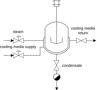
Direct heating and direct cooling jacket configuration

In this configuration the heating/cooling media enters directly into the jacket recirculation loop. The temperature of the heating/cooling media is quasi constant as it is controlled before entering the recirculation loop. Beside the previously mentioned advantages in contrast with the single pass solution, this configuration has a quick response time compared with the hereinafter described indirect solutions. The reason of the quick response time is the lack of any heat

steam

cooling media supply

condensate cooling media

return

(27)

exchangers between the heating/cooling media and the jacket recirculation that might make the heat transfer slower.

The configuration in Figure 1.2 is a multifluid, direct system with jacket recirculation. If the cooling media is water, depending on the pressure of the system the available temperature range is 5 – 180 °C. This jacket configuration with jacket ejector and recirculation was developed by Ciba-Geigy AG. The lower limit of the temperature range can be extended by using the mixture of water and ethyl-alcohol. The automation of the system is quite complicated as the changeover between the heating and cooling media can cause unwanted effects especially if controlling exothermic reactions. The heating/cooling media can contaminate each other during changeovers, which can also cause corrosion problems.

Figure 1.2: Direct heating and direct cooling jacket configuration Indirect heating and direct cooling jacket configuration

The temperature range of the indirect heating and direct cooling configuration is -20 – 180 °C. This type of configuration can be seen in Figure 1.3, where the heating is commonly achieved through a plate heat exchanger and the cooling is performed by the direct injection of the cooling media into the jacket recirculation loop. The changeover of the different modes can be performed smoothly using a split-range controller. Due to the direct cooling media injection the response time of the system is significantly lower in cooling mode. The advantage of this system is that there is no contamination due to changeover of the different fluids as only one type of fluid can enter the jacket recirculation loop. To achieve high temperature range, the cooling media must satisfy the requirements for heating purposes as well, since it transfers the heat from the heating heat exchanger to the reactor.

cooling media supply

condensate steam

cooling media return

(28)

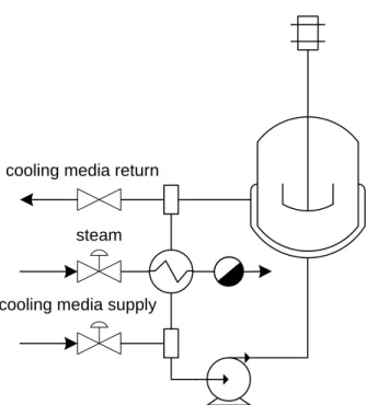
Figure 1.3: Indirect heating and direct cooling jacket configuration Indirect heating and indirect cooling jacket configuration

The indirect heating and cooling of the jacket recirculation loop can be achieved by two heat exchangers, one for the heating and one for the cooling media. This type of configuration can be seen in Figure 1.4. The advantage of this solution is that a cheaper cooling media can be used as it does not need to satisfy strict specifications compared with the previously described configurations. Also a centralized heat block service can be used for this solution providing the heating/cooling media for several reactors. The temperature range of this solution can reach -20 – 220 °C.

Figure 1.4: Indirect heating and indirect cooling jacket configuration

cooling media supply steam cooling media return

cooling media supply steam

(29)

Monofluid heating/cooling configuration

A quite different solution from the previously described ones is the monofluid heating/cooling configuration. It is a direct heating/cooling solution that contains a jacket recirculation loop, and the media used for heating and cooling has the same material quality. The reason behind the naming convention monofluid is the quality of the used media, which differs only in its temperature and not in quality. The production of the different temperature levels can be achieved by an independent thermoblock, which might provide heating/cooling media for several reactors. The widest temperature range available in this configuration is -30 – 360 °C that highly depends on the quality of the selected thermal fluid and the operating pressure of the monofluid thermoblock [8], [9].

Beside the advantages of the jacket recirculation loop configuration this solution has also a low response time due to the direct thermal fluid injection.

Also there is no changeover mechanism needed as the qualities of the different temperature levels are identical. This configuration has all the advantages of the direct and indirect solutions.

In a monofluid system where two temperature levels are used, the temperature control of the reactor can be achieved with a classical split-range controller. This control solution has several references in the literature and is identical to the ones used for the multifluid systems. However, more than two temperature levels can be used for the control of the reactor (also in the case of multifluid systems [10]) that require complex control mechanisms or advanced control solutions. Only a few publications are cited in the literature about systems containing a monofluid thermoblock with three different temperature levels and the split-range control for this configuration [7], [11], [12].

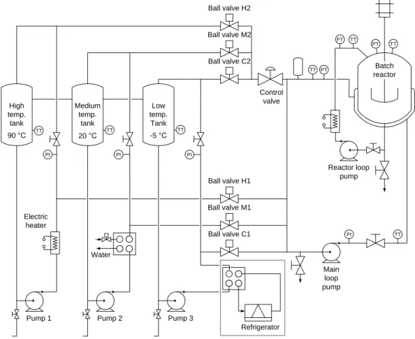
A solution connected with a monofluid thermoblock that contains three different temperature levels can be seen in Figure 1.5. The disadvantage of this configuration is that it needs the coordinated operation of the ball valves and the control valve to adjust the temperature of the jacket. The classical split-range solution is not capable to handle three temperature levels. However, this solution is more economic compared with solutions containing the two temperature levels.

It is more economical to use a medium temperature level that has a low operation cost than using only the more expensive temperature levels at the boundaries of the available temperature range. For example if the medium temperature level is controlled by water, which has a significantly lower operating cost than refrigeration, it is more preferable to use this level for the cooling of the reactor if temperature of the reactor is higher than the medium temperature level. However, to gain the advantages of this three-levelled system a control solution is also necessary that can utilize all the three levels.

(30)

Figure 1.5: Monofluid heating/cooling jacket configuration

1.2. Chemical Process Simulation

Establishing a chemical engineer pool with high base knowledge significantly depends on the quality of the education in the universities.

Instruction of chemical engineers should reflect the challenges they face in industry. Young chemical engineers are required to assimilate rapidly new and emerging technologies to react in a flexible manner to shorter production cycles and strict quality regulations [13]. A chemical engineer must have a working knowledge of mathematics, chemical and physical technology, biotechnology, materials science, and economics, which are the building blocks used by the design engineer. Additionally, competence in the use of the simulation tools allows process evaluation directly on an economic basis; controllability and operability can be assessed using dynamic simulation, while some simulation software automatically provides information to help determine the environmental impact of each of the product streams. Process simulators are an indivisible part of modern practice in chemical process design. Young engineers should have a well- structured knowledge relying on fundamentals as well as to have the balance between heuristic and computer-aided algorithmic approaches. The education should also reflect the current state-of-the-art in the integration of process design and process control. [14], [15], [16].

Chemical engineers have to make critical process and equipment design decisions in all stages of the process life-cycle, from the concept to the troubleshooting of an existing production process. In every stage different types of models with different information content are necessary to be used. This may range from the calculation of mass and energy balances of a single unit operation to the simulation and optimization of large flowsheets.

During the stages of a process life-cycle different models with different information content might be necessary [17]. In the phase of Research and Development (R&D) the form and accuracy of the models can first be quite simple, however it can become more detailed as work proceeds. The focus in R&D is in the phenomena: phase equilibrium, physical properties, chemical

high temp.

medium temp.

low temp.

high temp.

medium temp.

low temp.

(31)

into its components. The phenomena-related models then are combined into process unit models.

In the next step of the process life-cycle the conceptual design is performed.

The optimal process structure and operating conditions are searched in this stage;

the focus is on process synthesis and the full-scale plant. If the chemical components are well-known in the process, meaning usually that their properties and all related parameters can be found in databanks, models can be used to quickly check new process ideas. In distillation, design models are used to identify key and non-key components, the optimum distillation sequence, the number of ideal stages, feed stages, etc.

When a process reaches a step in its life-cycle where detailed engineering is applied, the focus is in technical solutions. Depending on the nature of the models, they can provide a description of how the system behaves in certain conditions, or they may be used to calculate detailed geometries of the equipment. When fine- tuned models are available the design of the new unit or process is easily optimized for yield or energy consumption.

The last phase in the life-cycle of the process is the operation stage. At this stage, models must include all relevant physical, chemical, and mechanical aspects. The model predictions are compared against actual plant measurements and tuned further to improve the accuracy of predictions. The focus at this stage is in guaranteeing optimal production. This is the stage where OTS (Operator Training Simulator) systems are applied. A detailed example can be found in the article of Zaldívar et al. [18], where the optimization of a batch reactor is achieved by using the simulator of the real process. Bradu et al. [19] describe the construction of an OTS system of a cryogenic plant that can be used for operator training, testing the control of the system, and plant optimization. Dynamic simulation has a very important role in such dynamic processes.

Today's process plants face all the real-world challenges to operational excellence; however, the stakes are much higher than ever before. The constantly changing nature of plants, and their internal and external environments, can threaten safe and profitable plant operations quickly. Uncontrolled upsets can cause start-up delays, production outages, severe equipment damage, and even catastrophic failures. The operational safety and excellence of the plant increasingly rely on well-trained, expert plant operators.

Dynamic Simulation and Operator Training Simulators have been available for a long time. However, over the last five years, improvements in technology (computers, software, and market understanding) have meant that the use of Dynamic Simulation and Operator Training Simulators has become a reality for many processes.

The primary OTS objectives are the following. The main objective is to keep the skilled workforce in spite of attrition by turnover or retirement, as it is one major prerequisite for a plant to operate safely and efficiently. The goal is to provide the plant operational staff with practical experience on how to operate complex plant process systems in various situations. Also an object of OTS systems is to assess the performance level of the trainees. [20]

(32)

High-tech automation is changing cognitive demands on operators, who are now required to:

 Supervise rather than directly monitor

 Make more cognitively complex decisions

 Deal with complex, mode-rich systems

 Increase need for cooperation and communication

An increasing number of chemical companies have recently decided to use OTS systems with the aim of training the operating staff on handling different plant failures, rarely used modes of operation, and measuring their skills. It is also an objective to support engineering tasks as well as testing new control methods and to perform safety tests without risk on the real system. [21], [22]

The main objectives of OTS use can be the following: [23]

 Practice procedures for plant start-up and shut-down situations

 Handling of utility system and process unit trips, turn-down, and other upsets

 Fault diagnosis, alarm handling, and corrective actions in case of process equipment malfunction during normal operation

 Practice steady-state operation

 Reduce start-up and shut-down times

 Increase safety

 Reduction in environmental concerns

 Increase unit up-time

 Increase operator awareness, skills, and readiness

 Assess operator competence

Optional functions of OTS systems:

 Testing and validation of operating procedures

 Testing and validation of control strategies and logic

 Debottlenecking

 Investigation of engineering solutions

 Sharing of incident and operating scenarios across shift teams

 Practicing energy efficient operation

 Understanding the operation of APCs

 APC limit handling and set-up

Computer-aided process design (CAPD) and simulation tools have been successfully used in chemical and oil industries since the early 1960s for the development and optimisation of integrated systems. Simulators used in these industries are designed to simulate continuous processes and their transient behaviour, mainly for process control purposes. Similar benefits can be achieved with the application of CAPD and simulation tools in other industries, such as