The effects of sensory quantization and control torque saturation on human balance control
Gergely Gyebr´ oszki
∗, G´ abor Csern´ ak
∗, John G. Milton
†, Tam´ as Insperger
‡§Peer-reviewed manuscript submitted at 2021.02.24.
Abstract
The effect of reaction delay, temporal sampling, sensory quantization and control torque saturation is investigated numerically for a single-degree-of-freedom model of postural sway with respect to stability, stabilizability and control effort. It is known that reaction delay has a destabilizing effect on the balancing process: the later one reacts to a perturbation the larger the possibility of falling. If the delay is larger than a critical value then stabilization is not even possible. In contrast, numerical analysis showed that quantization and control torque saturation have a stabilizing effect: the region of stabilizing control gains is larger than that of the linear model. Control torque saturation allows the application of larger control gains without overcontrol while sensory quantization plays a role of a kind of filter when sensory noise is present. These beneficial effects are reflected in the energy demand of the control process. On the other side, neither control torque saturation nor sensory quantization improve stabilizability properties. In particular, the critical delay cannot be increased by adding saturation and/or sensory quantization.
Aging western societies are facing an epidemic of falling [49]. For example, in the US an older adult is treated for a fall in the emergency room every 11 minutes and every 19 minutes an elderly person dies from a fall. Measurements of postural sway, namely the fluctuations in the center-of-pressure (COP) while a subject stands quietly on a force platform with eyes closed, can identify those most at risk for a fall [26, 70].
The principle sensory input for postural sway is proprioception at the ankle joint [15].
Since the sensory threshold for proprioception increases with aging and certain diseases which effect the nervous system (e.g. diabetic neuropathy), it has been suggested
∗Department of Applied Mechanics, Budapest University of Technology and Economics, Budapest, 1111, Hungary, e-mail: gyebroszki@mm.bme.hu, csernak@mm.bme.hu
†The Claremont Colleges, W. M. Keck Science Center, Claremont, CA 91711, USA, e-mail: JMil- ton@kecksci.claremont.edu
‡Department of Applied Mechanics, Budapest University of Technology and Economics and MTA-BME Lend¨ulet Human Balancing Research Group, Budapest, 1111, Hungary, e-mail: insperger@mm.bme.hu
§Corresponding author
that this sensory threshold increases the risk for falling [33, 49, 55]. Generalization of sensory dead zone is sensory quantization, which is a combination of a series of shifted sensory dead zones. However, mathematical and computer modeling studies suggest that sensory quantization can have stabilizing effects [12, 24, 32, 40, 42, 48, 60].
Computer simulations of an inverted pendulum model for balance stabilized by time- delayed feedback are used to assess the effects of sensory quantization on control effort [19, 20]. The results suggest that sensory quantization can slightly decrease control effort and that this benefit increases due to the effects of sensory masking to alter quantization thresholds [55]. These observations provide insights into the possible benefits of shoes with “noisy insoles” for reducing falling risk in elderly subjects [33].
1 Introduction
Falls in older adults typically occur while subjects are moving and are related to a variety of issues including weight transfer, slips and trips [56]. The lone exceptions are those falls related to disorders of the cardiovascular system (e.g. asystole, vasovagal episodes) and nervous system (e.g. spinal cord disease, intoxication, epileptic seizures). Thus it is counter-intuitive that measurements of postural fluctutations while standing quietly predict the propensity of an individual to fall while moving [26, 70].
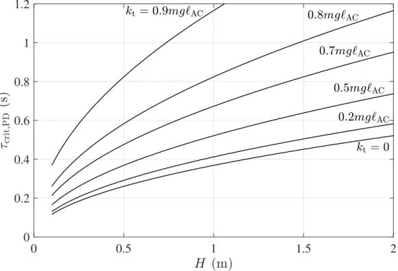
The dynamics exhibited by postural sway are very complex and consequently have attracted a great deal of attention [8, 12, 27, 36, 47, 38, 67, 68] Typically sway is modeled in terms of an inverted pendulum stabilized by time-delayed feedback [12, 27, 32, 38, 43, 59]. The time delay, τ, arises because it takes time for the nervous system to detect a deviation from vertical and then act upon it. A manifestation of the importance of τ for balance control is the observation that it is easier to balance longer poles at the fingertip than shorter ones [43]. The critical time delay, τcrit is the longest delay for which a pole of length `can be balanced. For proportional-derivative (PD) feedback, it is typically proportional to √
`. Figure 1 shows τcrit as a function of the length of the inverted pendulum in the model of postural sway for different passive ankle stiffness as discussed in Section 2. The time delay for human postural control is estimated to be between 100−200 ms [27, 32, 39, 50, 52, 53, 66]. The fact that τ < τcrit suggests that the critical delay does not set any limitation on models of postural control with delayed feedback.
The observations in Figure 1 suggest that instabilities in postural balance are most likely due to the limitations of the nervous system to detect deviations from vertical and/or the inability to generate sufficient ankle torque to correct displacements from vertical. The principle sensory input for postural sway is proprioception. Proprioceptive sensors at the ankle joint have a sensory threshold of ≈ 0.1◦ [15, 45] which is about 20% of the amplitude of postural sway. The sensory dead zone introduces a strong, small-scale nonlinearity into the control since the feedback is either on or off depending on whether the displacement angle is respectively, larger or smaller than the dead zone [12, 24, 41, 42]. A second strong nonlinearity arises because of saturation of the control torque at the ankle, i.e. the person may not be able to exert the required amount of torque at the ankle [9, 48, 54, 69]. Finally, experimental observations indicate that controlling forces are exerted intermittently [5, 36, 62]. This switching type of feedback may simply be a consequence of the sensory dead zone or part of the neural strategy for exerting control [1, 4, 18, 44, 50].
0 0.5 1 1.5 2 0
0.2 0.4 0.6 0.8 1 1.2
Figure 1: Critical delay as function of person’s height H(m) for different values of passive ankle stiffness kt (see equation (2)).
There have been two views of the roles played by a sensory dead zone in the control of human balance during quiet standing with eyes closed. The first considers that the sensory dead zone represents a threshold that must be overcome for effective control to occur. This point of view suggests the possibility of adding sensory stimuli to the soles of the feet to improve balance control by altering quantization thresholds [3, 57]. Indeed standing on a noisily vibrating platform [55] or wearing shoes with noisy insoles [33] decreases the amplitude of the fluctuations of human postural sway. The second considers that a sensory dead zone is necessary to avoid the deleterious effects of
“over-control” [32, 40, 44]. In this case the stabilizing effects of vibration on human balance arise from the interplay between the sensory dead zone and the time-delayed feedback [42].
Recently it has been shown that influences for balance control which are typically thought to be destabilizing, such as sensory quantization and muscle torque saturation, can actually be stabilizing when they work together [48]. Here we investigate the effects of sensory quantization and muscle torque saturation on a model of postural sway which includes “temporal sampling”.
The temporal sampling takes into the account the observation that the force generated by a muscle fiber depends on the frequency that it is stimulated at [11]. Our goal is to determine the control effort of this model as a function of sensory quantization and muscle torque saturation. Section 2 presents the model and Section 3 describes the main steps of the numerical analysis. Results on practical stability, critical delay and control effort are given in Section 4 and conclusions are drawn in Section 5.
2 Model
We model postural sway as an inverted pinned pendulum supported by a torsional spring and a torsional dashpot at the pivot point. Together the torsional spring and torsional dashpot represent the passive resistance of the ankle joint against falling. The mechanical model is shown in Figure 2.
The equation of motion is
JAθ(t) +¨ btθ(t) +˙ ktθ(t)−mg`ACsin(θ(t)) =−Q(t), (1) whereθ is the postural angle of the body measured from the upper (unstable) equilibrium position, θ˙and ¨θindicate its first and second derivative, JAis the moment of inertia of the body with respect to the ankle joint A, kt and bt are the torsional stiffness and the torsional damping at the ankle, respectively, m is the mass of the body, g is the gravitational acceleration, `AC is the distance between the center of gravity C and the suspension point A and Q(t) is the active control torque.
The passive resistance of the ankle joint is attributed to the foot, Achilles’ tendon and aponeurosis and cannot be regulated by the nervous system during quiet standing.
Linearization around the upright position gives
JAθ(t) +¨ btθ(t) + (k˙ t−mg`AC)θ(t) =−Q(t). (2) This form shows that the intrinsic ankle stiffness kt plays a key role in the stabilization process of upright stance [65]. If kt < mg`AC then the open-loop system is unstable. As shown by [35] for a group of fifteen healthy subjects, aged between 20 and 68 years, the passive ankle stiffness was substantially constant and was increasing only slightly with ankle torque, which verifies the linear
Figure 2: Mechanical model for postural sway during quiet standing in the anterior-posterior plane.
spring model. They found that nine out of the fifteen subjects had kt < mg`AC and the average of the ratio kt/mg`AC for the fifteen subjects was 0.91 with standard deviation 0.23. Other studies used slightly different values for kt/mg`AC ranging between 0.5∼0.9 [38, 1, 61, 29]. These studies indicate that the intrinsic mechanical stiffness of the ankle is just not enough to stabilize passively the upright stance. Thus active feedback control is required to guarantee stability.
The active feedback is most often assumed to be a delayed PD feedback of the form [27, 32, 38, 47, 50, 52, 59]
Q(t) = Kpθ(t−τ) +Kdθ(t˙ −τ), (3) whereKpandKd are the proportional and the derivative feedback gains andτ is the reaction delay.
Substituting (3) into (2) and dividing by JA gives
θ(t) +¨ bθ(t) +˙ aθ(t) =−kpθ(t−τ)−kdθ(t˙ −τ), (4) where
b= bt
JA , a= kt−mg`AC
JA <0, (5)
kp = Kp
JA , kd = Kd
JA . (6)
In what follows, the parameters are set as shown in Table 1 following the paper by Asai at al.
[1]. The intrinsic damping parameter bt of the ankle joint is the most uncertain parameter in the model, estimates in the literature range between 4 ∼500 Nms/rad [1, 52, 39] and it is often simply set to zero [48, 29]. It should also be noted that bt does not contribute to the passive stabilization directly since the only condition for stability is bt ≥0.
Table 1: Parameters mh 60 kg
JA 60 kgm2
`AC 1 m
kt 470 Nm/rad (80% of mg`AC) bt 4 Nms/rad (will be set to zero)
2.1 Linear stability
The stability criteria for the system can be derived by means of the D-subdivision method [58, 59].
The characteristic function reads
D(λ) = λ2+bλ+a+kpe−λ+kdλe−λ . (7) Substitution of λ= jω gives the D-curves in the form
if ω = 0 : kp =−a , kd ∈R, (8)
if ω 6= 0 :
(kp = (ω2−a) cos(ωτ) +bωsin(ωτ),
kd = ω2ω−asin(ωτ)−bcos(ωτ). (9) Characteristic exponents can exist on the imaginary axis only along the D-curves. Thus the number of unstable characteristic exponents is constant within the regions separated by the D-curves. The stable region is the one associated with zero unstable characteristic exponents.
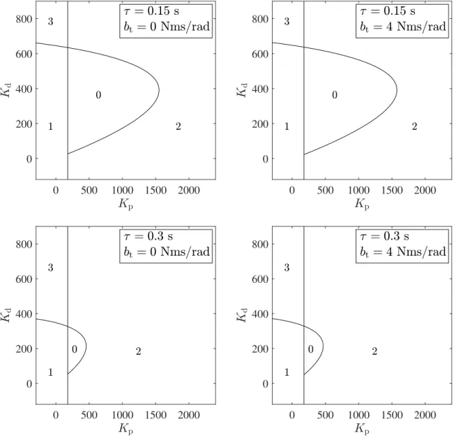
Stability diagrams and the number of unstable characteristic exponents are shown in Figure 3.
The parameters correspond to those in Table 1. It can be seen that the stable region does not typically change as the damping is increased from 0 to 4 Nms/rad (which is the value suggested by Asai et al.[1]), while the change is more relevant with the change of the delay. This observation highlights that the delay parameter is more relevant with respect to the stabilizability than the damping term.
2.2 Critical delay
As can be seen in Figure 3, the stable region shrinks with the increase of the delay. When the tangent of the parametric curve (9) becomes vertical at ω = 0 then the stable region totally disappears. It can be shown that this happens when
aτ2+ 2bτ + 2 = 0, (10)
hence the critical delay is
τcrit,PD =−1 a
b+√
b2−2a
. (11)
Ifτ > τcrit,PD then the system cannot be stabilized by delayed feedback for anykp andkd. If bt = 0 then τcrit,PD = 1.0096 s, if bt = 4 Nms/rad then τcrit,PD = 1.0442 s. This shows that bt does not
0 500 1000 1500 2000 0
200 400 600 800
0 500 1000 1500 2000 0
200 400 600 800
0 500 1000 1500 2000 0
200 400 600 800
0 500 1000 1500 2000 0
200 400 600 800
Figure 3: D-curves and the number of unstable characteristic roots for (4) for different delays and different intrinsic ankle damping.
affect stabilizability for the relevant parameter regions. In the discussion which follows we assume that bt (and hence b) is equal to zero.
If the human body is modeled as a homogeneous rod with JA = 13mH2 and `AC = 12H with H being the height of the person and kt = 0.8mg`AC, then one gets a rough estimate for the critical delay as function of the person’s height H as
τcrit,PD = r 2
−a = s
20H
3g . (12)
2.3 Spatial and temporal quantization
When temporal quantization (‘sampling effect’) is taken into account then the governing equation reads
θ(t) +¨ bθ(t) +˙ aθ(t) =−kpθ(tj −r∆t)−kdθ(t˙ j−r∆t), t∈[tj, tj+1), (13) where tj =j∆t are the sampling instants and ∆t is the sampling period such that τ =r∆t. Here, we take ∆t= 10 ms.
Sensory quantization is a simplified model of the inaccuracies of human sensory perception, namely, the feature that small changes in sensory input are not followed by changes in the output.
For instance, 1.2◦ and 1.3◦ angular excursion may induce the same corrective action, but when the angle exceeds, e.g., 1.5◦ then larger action is triggered. When spatial quantization of the perceived sensory signals are also modeled, then the equation changes to
θ(t) +¨ bθ(t) +˙ aθ(t)
=−kpρpInt 1
ρpθ(tj −r∆t)
−kdρvInt 1
ρv
θ(t˙ j−r∆t)
,
t ∈[tj, tj+1), (14) where ρp and ρv are the quantization step of the perceived angular position θ and the perceived angular velocity ˙θ, respectively. The sensory quantization has been implemented using the function Int( ) which rounds towards zero, e.g., Int(1.6) = 1, Int(−1.6) = −1 [46, 47, 60, 20]. Note that Int(x) = 0 if −1 < x < 1, therefore sensory quantization also presents a sensory dead zone when the system is close to the equilibrium. The size of sensory quantization for human perception is a debate of questions [15, 40, 32, 46]. Here we reduce our analysis to ρp < 8◦ and ρv <8◦/s. In the following, (14) is analyzed numerically. Particularly, the stability and stabilizability properties, and the control effort are determined for different time delays and quantization steps.
2.4 Control torque saturation
Falling is often associated to the saturation of the control torque, i.e., the subjects cannot exert the required amount of torque at their ankle (see, for example, [7, 54]. From a dynamics point of view, control torque saturation presents strong nonlinearity associated with subcritical bifurcation which reduces the domain of attraction of the stabilized fixed point [69]. The governing equation
for the model which takes into account saturation is θ(t) +¨ bθ(t) +˙ aθ(t) = 1
JA
Q(t)˜ , (15)
where
Q(t) =˜
Qmax if Q(t)≥Qmax Q(t) if |Q(t)|< Qmax
−Qmax if Q(t)≤ −Qmax
(16)
and
Q(t) = −KpρpInt 1
ρpθ(tj −r∆t)
−KdρvInt 1
ρv
θ(t˙ j −r∆t)
,
t ∈[tj, tj+1). (17) Here Qmax is the maximum exertable control torque, which, following [48], is taken to be Qmax = 20 Nm. Note that the factor 1/JA in (15) is compensated by using Kp and Kd in (17) according to (6).
2.5 Limitation by basin of support
Maintaining static balance is not possible if the projection of the centre of mass to the ground is outside of the basin of support. Assuming an average foot length of 28 cm with `AC = 1 m, one gets the limiting angle θlim ≈ 8◦. We assume the balance is lost at time instant t = tfall when
|θ(tfall)|> θlim.
2.6 Control effort
The energy demand of the control process for each simulation was calculated as E =
Z tmax
0
Q(s) ˙θ(s)
ds . (18) Clearly, one control goal is the minimization of the energy during balancing. For numerical calcu- lations, the time duration was set to tmax = 100 s.
3 Numerical method
The solution for (15) with (16) and (17) was determined numerically for a set of control gains (kp, kd) and for different quantization stepsρpand ρv. Since the right hand side of (15) is piecewise constant, the solution over each sampling period can be given in closed form using the variation of constants formula. Step-by-step solution over the succeeding sampling periods gives a discretized time history ofθand ˙θover the interval [0, tmax]. The system parameters were set according to Table 1, the damping was set to b = 0. Simulations were performed for four different initial conditions:
(θ(0),θ(0)) = (ρ˙ p,0), (ρp, ρv), (0, ρv), (ρp,−ρv) such that |θ(s)|< ρp and |θ(s)|˙ < ρv for s ∈[τ,0].
Thus, the simulations were started from the ‘edge’ of the sensory dead zone, and the history function did not have any affect on the solution. Note that the initial conditions (θ(0),θ(0)) = (−ρ˙ p,0), (−ρp,−ρv), (0,−ρv), (−ρp, ρv) give the same response but with opposite sign. Simulations were terminated either after tmax= 100 s or when the angular position exceeded θlim.
Diagrams of practical stability were determined by running simulations for a fixed delay and for fixed spatial quantization steps over the plane of the control gains (kp, kd). The control gains were varied between Kp = 0 ∼ 1000 Nm/rad and Kd = 0 ∼ 1000 Nms/rad. Those control gain pairs were assessed as practically stable where the balance time exceededtmax with|θ(s)|< θlimfor s∈[0, tmax].
Stabilizability diagrams were determined as follows. First, the spatial quantization steps were fixed between the values ρp = 0 ∼ 10◦ and ρv = 0 ∼ 15◦/s. Then the maximum delay for which none of the simulations resulted in a fall was determined over the three-dimensional space (kp, kd, τ) using the multi dimensional bisection method [2]. The critical delay was determined as the delay τcrit =rcrit∆t, for which the simulation was stable for tmax, but for τ = (rcrit+ 1)∆t the simulation was not stable any more (i.e., |θ(s)| exceeded θlim). For a given pair of spatial quantization, the critical delay was set to the maximum of the delay that could be achieved over the plane (kp, kd).
4 Results
Stability, stabilizability (i.e., critical delay) and control effort were investigated based on the nu- merical simulations.
4.1 Practical stability
In order to show the effect of spatial quantization and control torque saturation separately, simu- lations were performed with and without quantization and saturation. The corresponding stability diagrams are shown in Figure 4. Grey and blue regions correspond to practically stable system, i.e., when |θ(s)| < θlim for s ∈ [0, tmax] in all simulations with different initial conditions. In the grey region, the control force was not saturated at all, i.e., |Q(s)|< Qmaxfors ∈[0, tmax] in all sim- ulations. In the blue region the control force was saturated at least in one sampling instant during the simulation. In the white region, the solution was not practically stable. Black line indicates the stability boundaries of the linear system, i.e., without spatial quantization and without control torque saturation, for reference. Figure 4 compares four cases.
• When there are no quantization (ρp = 0 and ρv = 0) and no saturation (Qmax = ∞), then the practically stable region coincides with the region of linear stability. The small difference between the two boundaries is due the temporal discretization [25].
• When there is saturation but no quantization (ρp = 0, ρv = 0), Qmax = 20 Nm), then the stable region opens up for larger control gains compared to the linear model. In this case, application of large control gains do not result in over control due to the saturation.
Figure 4: Regions of practical stability with (bottom) and without (top) quantization and with (right) and without (left) saturation for τ = 200 ms. Grey region: bounded solution such that Q does not exceed the saturation limit Qmax. Blue region: bounded solution such that Q is actually saturated.
• When there is quantization but no saturation (ρp= 1◦,ρv = 1◦/s),Qmax =∞), then the size of the stable region is again larger than that of the linear model.
• The case when both quantization and saturation are present (ρp = 1◦, ρv = 1◦/s, Qmax = 20 Nm) gives a combination of the previous two cases. The stable region is the largest in this case.
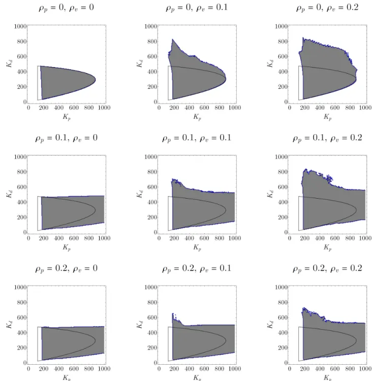
The effects of different quantization steps is illustrated in Figure 5 for Qmax = 20 Nm. As can be seen, the size of the practically stable regions slightly increases when spatial quantization is larger. On the other side, it can also be seen that for larger quantization steps the saturation-free region (grey region) is smaller.
4.2 Critical delay
The critical delay over the plane of the spatial quantization (ρp, ρv) is shown in Figure 6. It can be seen that the maximum critical delay is obtained for zero quantization. Thus, although the size of the stable region increases due to the quantization, the critical delay cannot be increased by adding quantization. This result is similar to that of the quantized Hayes equation (a first-order delay
Figure 5: Regions of practical stability for different quantization steps (ρp, ρd) forτ = 200 ms and Qmax = 20 Nm.
(ms)
Figure 6: Critical delay as function of quantization steps (ρp, ρd) forQmax = 100 Nm.
equation) in [60]. Note that small fragmentation in the surface plot is due to the finite resolution of the parameters space used during the numerical calculations.
4.3 Control effort
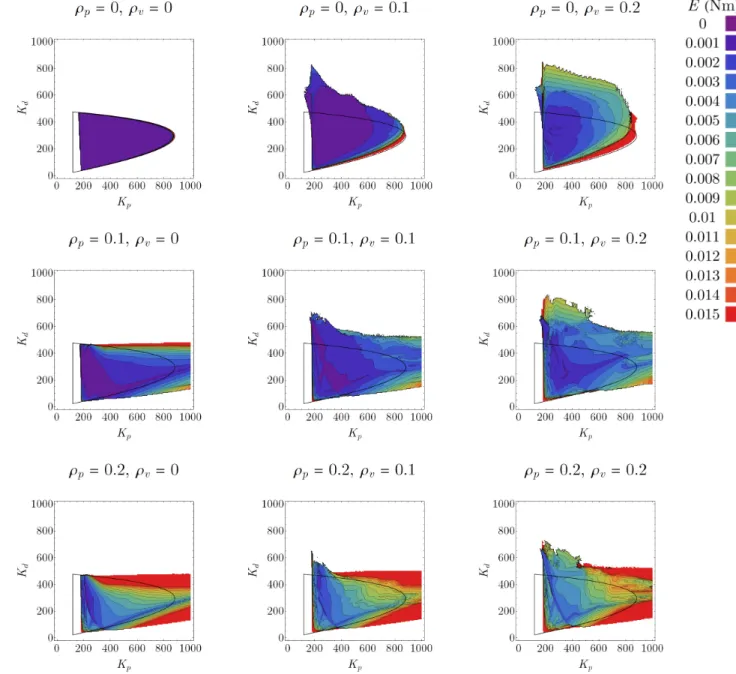
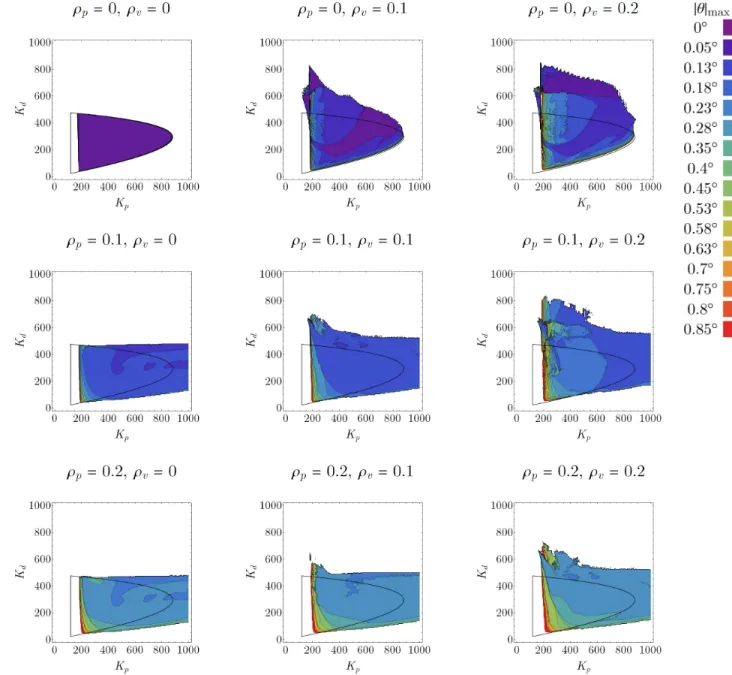
Control effort over the plane of the control gains for different spatial quantizations is shown in Figure 7. Different levels of control energy E are shown by different color. The unstable region is indicated by red color. Small control energy is indicated by blueish (from blue to purple) colors.
It can be seen that the smallest control energy is required in the stable region of the quantization- free case. The reason for this is that the corresponding ideal motion is exponentially decaying.
Besides this, there are some parameter regions, where the quantization reduces the control effort.
For instance the blue region (low energy region) in the case ρp = 1◦, ρv = 1◦/s, is larger than in the case ρp = 1◦, ρv = 0◦/s. The orange region (large energy region) disappears when there is quantization in the velocity. Thus, we can conclude that quantization slightly decreases control effort in certain parameter regions. Note that the colorbar in Figure 7 corresponds to a logarithmic scale.
4.4 Size of postural sway
An important feature of postural sway is the size of the oscillations. Figure 8 shows the maximum values of the fluctuations during the simulations for the same parameters as in Figure 7. It can be seen that the oscillations are larger in the lower left region of the stability diagrams when ρp >0 and ρv>0 (this can be observed especially forρp= 2◦ and ρv= 2◦/s). A combination of Figures 7 and 8 suggest that the control gains are tuned by optimizing a combination of control effort and resulted oscillations.
Figure 7: Distribution of the control effort in the space of control gains and quantization steps for reaction delay τ = 200 ms.
Figure 8: Maximum of the fluctuations obtained by numerical simulations for reaction delay τ = 200 ms.
5 Discussion
Sensory quantization and control torque saturation are unavoidable elements of control systems due to physical limits in sensory perception and in actuation. In human balancing, finite resolution of perception and maximum exertable effort can also be described in terms of quantization and saturation. Moreover, it is also necessary to take into account temporal sampling since the corrective forces generated by muscle contractions depend on the frequency of discrete neural inputs. Acting together these effects can produce low-amplitude chaotic or at least seemingly chaotic vibrations that resemble the random-like motion during postural sway [30, 50, 31, 60, 47]. Both quantization and saturation have a beneficial effect on the performance. Quantization does not allow reactions to perturbations that are smaller than the quantization step, hence, it serves as a kind of filter to reduce noise [37]. One of the simplest realization of quantization is sensory dead zone: a threshold below which changes in sensory input are not reflected by changes in output. Saturation prevents overcontrol [48], which means that large control gains can be used without actually generating large control action. An extreme case of the control torque saturation result in a bang-bang control: the control torque is switched between two constant values [12, 25].
Sensory quantization decreases the control effort for stabilizing balance during quiet standing.
The beneficial effects of noisy insoles on balance [33, 55] is thought to be mediated through the effects of sensory masking to alter the threshold for sensory quanization [55]. The benefits of sensory quantization do not increaseτcrit, but rather makes the control more robust in the presence of fluctuations in the control gains. It is difficult to attribute these effects to a benefit of noise per se since about 80 % of the amplitude fluctuations are greater than the sensory threshold. Thus it appears that it is the saturation of muscle torque together with sensory quantization that provides the main benefits for control. The tendency of the effect of quantization, saturation and their combination can be seen in Figure 4. The control torque is saturated in the blue region, which shows that the extension of the region of practical stability to large control gains is indeed related to saturation.
The control gains which are most robust in the face of stochastic fluctuations, sensory quanti- zation and control torque saturation are those located in the left corner of the D-shaped stability region in the plane of the control gains. Similar observations have been obtained for pole balancing at the fingertip [46], virtual pole balancing [28], and in studies of the effects of structured, real perturbations on postural sway [21]. Estimations of the control gains for standing balance obtained by modeling the responses to mechanical perturbation also place the control gains in this same regions of parameter space (A. Zelei, J. Milton, G. Stepan and T. Insperger, in preparation). The reason why the employed control gains are located not exactly on the edge of the stability region is that the resulted oscillations for small gains are larger as shown in Figure 8. The magnitude of the oscillations is smaller for larger control gains. Hence, the actual control gains applied might be a result of a trade-off between small control effort and small fluctuations.
Our observations support two beneficial proposal for stabilizing standing balance in the elderly:
1) increase the torque that can be exerted across the ankle joint, and 2) addition of noisy perturba- tions. It is important to keep in mind that both of these benefits can be implemented non-invasively.
It is likely that increasing ankle torque would provide the most benefit; however, our results do not eliminate the possible benefits of wearing footwear with noisy insoles [33, 55]. However, it must be kept in mind that these benefits are small and do not reverse the effects of aging. Of course the
major unsolved problem is understanding how these effects reduce the risk of falling while moving.
Acknowledgement
The research reported in this paper and carried out at BME has been supported by the Hungarian National Research, Development and Innovation (NRDI) Office under Grant No. NKFI-128422.
(GG, GC), by the NRDI Fund (TKP2020 IES, Grant No. BME-IE-BIO and TKP2020 NC, Grant No. BME-NC) based on the charter of bolster issued by the NRDI Office under the auspices of the Ministry for Innovation and Technology (GG, IT, GC) and from the William R Kenan, Jr Charitable trust (JM).
Data Availability Statement
The data that support the findings of this study are available from the corresponding author upon reasonable request.
References
[1] Y. Asai, Y. Tanaka, K. Nomura, T. Nomura, M. Casidio and P. Morasso. A model of postural control in quiet standing: robust compensation of delay-induced instability using intermittent activation of feedback control. PLoS ONE, 4: e6169, 2009.
[2] D. Bachrathy and G. Stepan. Bisection method in higher dimensions and the efficiency num- ber. Period. Polytech. Mech. Eng., 56: 81–86, 2012.
[3] S. J. Bolanowski, G. A. Gescheider, R. T. Verrillo and C. M. Checkosky. Four channels mefiate the mechanical aspects of touch. J. Acoust. Soc. Am., 85: 1680-1694, 1988.
[4] A. Bottaro, Y. Yasutake, T. Nomura, M. Casidio and P. Morasso. Bounded stability of the quiet standing posture: an intermittent control model. Hum. Mov. Sci., 27: 473-495, 2008.
[5] J. L. Cabrera and J. G. Milton. On-off intermittency in a human balancing task. Phys. Rev.
Lett., 89: 158702, 2002.
[6] T. Chen and B. A. Francis.Optimal Sampled-Data Control. Springer-Verlag, New York, 1995.
[7] Choi J-H and Kim N-J. 2015. The effects of balance training and ankle training on the gait of elderly people who have fallen. J. Phys. Ther. Sci. 27, 139-142.
[8] J. J. Collins and C. J. De Luca. Random walking during quiet standing. Phys. Rev. Lett., 73:
764-767, 1994.
[9] R. G. Crilly, D. A. Williams, K. J. Trenholm, K. C. Hayes and L. F. O. Delaquerri´ere- Richardson. Effect of exercise in postural sway in the elderly.Gerontology, 35: 137-143, 1989.
[10] D. F. Delchamps. Stabilizing a linear system with quantized state feedback. IEEE Trans.
Automatic Control, 35, 916-924, 1990.
[11] R. M. Enoka and J. Duchateau. Rate coding and the control of muscle force. Cold Spring Harbor Perspectives Med., 7: a029702, 2017.
[12] C. W. Eurich and J. G. Milton. Noise-induced transitions in human postural sway.Phys. Rev.
E, 54: 6681-6684, 1996.
[13] S. Fauve and F. Heslot. Stochastic resonance in a bistable system. Phys. Lett. A, 97: 5-7, 1983.
[14] O. Feely. A tutorial introduction to non-linear dynamics and chaos and their applications to sigmadelta modulation. Int. J. Circ. Theor. Appl., 25: 347-367, 1997.
[15] R. Fitzpatrick and D. I. McCloskey. Proprioceptive, visual and vestibular thresholds for the perception of sway during standing in humans. J. Physiol., 478: 173-186, 1994.
[16] I. Fl¨ugge-Lotz. Discontinuous and optimal control. McGraw-Hill, New York, 1968.
[17] L. Gammaitoni, P. H¨anggi, P. Jung and F. Marchesoni. Stochastic resonance. Rev. Mod.
Phys., 70: 223-288, 1998.
[18] P. Gawthrop, I. Loram, H. Gollee and M. Lakie. Intermittent control models of human stand- ing: similarities and differences. Biol. Cybern., 108: 159-168, 2014.
[19] G. Gyebr´oszki and G. Csern´ak. Twofold quantization in digital control: deadzone crisis and switching line collision. Period. Polytech. Mech. Eng., 63(2):148–155, 2019.
[20] G. Gyebr´oszki and G. Csern´ak. The hybrid micro-chaos map: digitally controlled inverted pendulum with dry friction. Nonlinear Dyn., 98:1365–1378, 2019.
[21] D. Hadju, J. Milton and T. Insperger. Extension of stability radius to neuromechanical sys- tems with structured real perturbations. IEEE Trans. Neural Syst. Rehab. Eng., 24: 1235- 1342, 2016.
[22] G. Haller and G. St´epan. Micro-chaos in digital control. J. Nonlinear Sci., 6: 415-448, 1996.
[23] T. Insperger. Stick balancing with reflex delay in case of parametric forcing.Commun. Nonlin.
Sci., 16: 2160-2168, 2001.
[24] T. Insperger, J. Milton and G. Stepan. Acceleration feedback improves balancing against reflex delay. J. R. Roy. Interface, 10: 20120763, 2013.
[25] T. Insperger, J. Milton and G. Stepan. Semidiscretization for time-delayed neural balance control. SIAM J. Dyn. Sys., 14: 1258-1277, 2015.
[26] J. Johansson, A. Nordstr¨om, Y. Gustafson, C. Westling and P. Nordstr¨om. Increased postural sway during quiet standing as a risk factor for prospective falls in community-dwelling elderly individuals. Age Ageing, 46: 964-070, 2017.
[27] T. Kiemel, K. S. Oie and J. J. Jeka. Slow dynamics of postural sway are in the feedback loop.
J. Neurophysiol., 95: 1410-1418, 2005.
[28] B. A. Kovacs, J. Milton and T. Insperger. Virtual stick balancing: Sensory uncertainties in angular displacement and velocity. Roy. Soc. Open Sci., 6: 191006, 2019.
[29] C. Le Mouel and R. Brette. Anticipatory coadaptation of ankle stiffness and sensorimotor gain for standing balance. PLoS Comput. Biol., 15(11): e1007463.
[30] L. Ladislao and S. Fioretti. Nonlinear analysis of posturographic data. Med. Bio. Eng. Com- put. 45, 679 (2007).
[31] K. Liu, H. Wang, J. Xiao and Z. Taha. Analysis of human standing balance by largest Lyapunov exponent. Comp. Intelligence Neurosci.2015, 158478 (2015).
[32] Y. Li, W. S. Levine and G. E. Loeb. A two-joint human postural control model with realistic neural delays. IEEE Trans. Neural Syst. Rehab. Eng., 20: 738-748, 2012.
[33] L. Lipsitz, M. Lough, J. Niemi, T. Travison, H. Howlett and B. Manor. A shoe insole delivery subsensory vibration noise improves balance and gait in elderly healthy people. Arch. Phys.
Med. Rehabil., 96: 432-439, 2015.
[34] A. Longtin, A. Bulsara and F. Moss. Time interval sequences in bistable systems and the noise induced transmission of information by sensory neurons.Phys. Rev. Lett., 67: 656-659, 1991.
[35] I. D. Loram and M. Lakie. Direct measurement of human ankle stiffness during quiet standing:
the intrinsic stiffness is insufficient for stability. J. Physiol., 545: 1041-1053, 2002.
[36] I. D. Loram, C. N. Maganaris and M. Lakie. Human postural sway results from frequent, ballistic bias impulses by soleus and gastrocnemius. J. Physiol., 564: 295-311, 2005.
[37] M. W. Marcellin and M. A. Lepley and A. Bilgin and T. J. Flohr and T. T. Chinen and J. H.
Kasner. An overview of quantization in JPEG 2000. Signal Proc. Image Commun.17, 73–84.
[38] C. V. Maurer and R. J. Peterka. A new interpretation of spontaneous sway measures based on a simple model of human postural control. J. Neurophysiol., 93: 189-200, 2005.
[39] K. L. McKee and M. C. Neale. Direct estimation of the parameters of a delayed, intermittent activation feedback model of postural sway during quiet standing. PLoS ONE, 14: e0222664, 2019.
[40] J. G. Milton, J. L. Cabrera and T. Ohira. Unstable dynamical systems: Delays, noise and control. Europhysics Lett., 83: 48001, 2008.
[41] J. Milton, J. L. Townsend, M. A. King and T. Ohira. Balancing with positive feedback: the case for discontinuous control. Philos. Trans. R. Soc., 367: 1181-1193.
[42] J. G. Milton, T. Ohira, J. L. Cabrera, R. M. Fraiser, J. B. Gyorrfy, F. K. Ruiz, M. A. Strauss, E. C. Balch, P. J. Marin and J. L. Alexander. Balancing with vibration: a prelude for “drift and act” control. PloS ONE, 4: e7427, 2009.
[43] J. G. Milton, J. L. Cabrera, T. Ohira, S. Tajima, Y. Tonosaki, C. W. Eurich and S. A.
Campbell. The time-delayed inverted pendulum: Implications for human balance control.
Chaos, 19: 026110, 2009.
[44] J. G. Milton. Intermittent motor control: The “drift and act” hypothesis. In: Progress in Motor Control: Neural, computational and dynamic approaches (M. J. Richardson, M. Riley and K. Shockly, eds). Springer, New York, pp. 169-193, 2013.
[45] J. Milton, T. Insperger and G. Stepan. Human balance control: Dead zones, intermittency and microchaos. In: Mathematical approaches to biological systems: Networks, oscillations and collective phenomena(T. Ohira and T. Ozawa, eds), Springer, New York, pp. 1-28, 2015.
[46] J. Milton, R. Meyer, M. Zhvanetsky and T. Insperger, Control at stability’s edge minimizes energetic costs: expert stick balancing. J. R. Soc. Interface, 13: 20160212, 2016.
[47] J. G. Milton, T. Insperger, W. Cook, D. M. Harris and G. Stepan. Microchaos in human postural balance: sensory dead zones and sampled time-delayed feedback. Phys. Rev. E, 98:
022223, 2018.
[48] J. Milton and T. Insperger. Acting together, destabilizing influences can stabilize human balance. Phil. Trans. R. Soc. A, 377: 20180126, 2019.
[49] F. Moss and J. Milton. Balancing the unbalanced. Nature, 425: 911-912, 2004.
[50] T. Nomura, S. Oshikawa, Y. Suzuki, K. Kiyone and P. Morasso. Modeling human postural sway using an intermittent control and hemodynamic perturbations.Math. Bioci., 245: 86-95, 2013.
[51] T. Ohira and J. G. Milton. Delayed random walks. Phys. Rev. E, 52: 3277-3280, 1995.
[52] J. H. Pasma, T. A. Boonstra, J. van Kordelan, V. V. Spyropoulou and A. C. Schouten. A sensitivity analysis of an inverted pendulum balance control model.Front. Comput. Neuroci., 11: 99, 2017.
[53] R. J. Peterka. Sensorimotor integration in human postural control. J. Neurophysiol., 88:
1097-1118, 2002.
[54] M. Pijnappels, N. D. Reeves, C. N. Marganaris and J. van Die¨en. Tripping without falling:
lower limb strength, a limitation for balance recovery and a target for training in the elderly.
J. Electromyogr. Kinesiol., 18: 188-196, 2008.
[55] A. Priplata, J. Niemi, M. Salen, J. Harry, L. A. Lipsitz and J. J. Collins. Noise-enhanced human balance control. Phys. Rev. Lett., 89: 238101, 2002.
[56] S. N. Robnovitch, F. Feldman, Y. Yung, R. Schonnop, R. P. M. Leung, T. Sarraf, J, Sims- Gould and M. Loughlin. Video capture of the circumstances of falls in elderly people residing in long term care: an observational study. Lancet, 381: 47-54, 2012.
[57] S. Ryu, D. Pyo, S.-C. Lim and D.-S. Kwon. Mechanical vibration influences the perception of electrovibration. Sci. Rep., 8:4555, 2018.
[58] G. Stepan. Retarded dynamical systems. Longman, Harlow, 1989.
[59] G. Stepan. Delay effects in the human sensory system during balancing. Phil. Trans. Roy.
Soc. A, 367: 1195-1212, 2009.
[60] G. Stepan, J. G. Milton and T. Insperger. Quantization improves stabilization of dynamical systems with delayed feedback. Chaos, 27: 114306, 2017.
[61] Y. Suzuki, T. Nomura, M. Casadio, P. Morasso. Intermittent control with ankle, hip, and mixed strategies during quiet standing: A theoretical proposal based on a double inverted pendulum model. J. Theo. Biol., 310(2012): 55-79.
[62] Y. Suzuki, A. Nakamura, M. Milosevic, K. Nomura, T. Tanahashi, T. Endo, S. Sakoda, P.
Morasso and T. Nomura. Postural instability via a loss of intermittent control in elderly and patients with Parkinson’s disease: A model-based and data-driven approach.Chaos, 30:
113140, 2020;
[63] T. Ushio and K. Hirai. Chaotic behavior in piecewise-linear sampled data control systems.
Int. J. Non-Linear Mech., 20: 493-506, 1985.
[64] D. A. Winter.Biomechanics and Neural Control of Human Movements, 4th edition. J. Wiley
& Sons, New York, 2009.
[65] D. A. Winter, A. E. Patla, F. Prine, M. G. Ishac and K. Gielo-Perczak. Stiffness control of balance during quiet standing. J. Neurophysiol., 80: 1211-1221, 1998.
[66] M. H. Woollacott, C. van Hosten and B. R osblad. Relation between muscle response onset and body segmental movements during postural perturbations in humans. Exp. Brain Res., 72: 593-604, 1986.
[67] N. Yamada. Chaotic swaying of the upright posture. Hum. Mov. Sci., 14: 711-726, 1995.
[68] V. M. Zatsiorsky and M. Duarte. Rambling and trembling in quiet standing. Motor Control, 4, 185-200, 2000.
[69] L. Zhang, G. Stepan and T. Insperger. Saturation limits the contribution of acceleration feedback to balancing against reflex delay. J. R. Soc. Interface, 15: 20170771, 2018.
[70] J. Zhou, D. Habtemariam, I. Iloputaife, L. A. Lipsitz and B. Manor. The complexity of standing postural sway associates with future falls in community-dwelling older adults: the MOBILIZE Boston study. Sci. Rep., 7, 2924, 2017.