Transient stabilization of an inverted pendulum with digital control
Gergely Geza Lublovary∗,Tamas Insperger∗
∗Department of Applied Mechanics, Budapest University of Technology and Economics and MTA-BME Lend¨ulet Human Balancing Research
Group, Budapest, Hungary (e-mail: lublovarygergo@gmail.com, insperger@mm.bme.hu)
Abstract: A possible explanation for a transient behavior of digitally controlled machines is presented. The mechanical system under study is an inverted pendulum controlled by a reaction wheel. A proportional-derivative feedback is used to control the unstable equilibrium of the pendulum. Modeling the quantization and the saturation of the applied control torque shows that these strong nonlinearities may change the local behavior of the system. Namely, control gains associated with a linearly unstable system can be stabilizing in the presence of control torque saturation. The results are demonstrated on an experimental device.
Keywords:digital control, feedback delay, stabilization, transient chaos 1. INTRODUCTION
Stabilization of motions about a desired trajectory is a key task in robotic manipulators. Correction of the deviations from the desired path requires a feedback mechanism, which inherently involves a dead time (feedback delay) due to the finite-time signal processing and transformation (Gorinevsky et al., 1997; Stepan, 2001; Hu and Wang, 2002). Time delay is often considered as an unwanted fea- ture of feedback systems, which is responsible for poor per- formance and may even destabilize the closed loop system.
Car-following-traffic models (Zhang et al., 2018), network dynamics (Otto et al., 2018), crane payload stabilization (Erneux and Kalmar-Nagy, 2007), control of machine tool chatter (Lehotzky et al., 2018; Munoa et al., 2013) and digital position control (Stepan, 2001; Habib et al., 2017) are examples of practical applications. Proper design of the control parameters is therefore of key importance.
Control systems are often designed based on linear models but their realizations involve many strong nonlinearities, such as quantization or saturation of the actuator signal.
The realization therefore may show different behavior than the underlying linear model (Ushio and Hsu, 1987;
Delchamps, 1990). Combination of quantization (spatial discretization) with the sampling effect of the digital controller (temporal discretization) may result in chaotic behavior (Stepan et al., 2017). Simple numerical examples show that permanent or transient chaos may show up for parameters, for which the system is linearly unstable.
The current paper was motivated by an experimental balancing device, an inverted pendulum equipped with a reaction wheel, which showed the phenomenon of tran- sient stabilization. The pendulum is stabilized with small oscillations about its upper equilibrium for a while, then, at some unpredictable time, the pendulum falls. The phe- nomenon is investigated using a mechanical model with quantization, saturation and digital sampling.
2. MECHANICAL MODEL
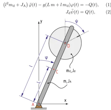
The mechanical model of the inverted pendulum is shown in Fig. 1. The control torqueQis provided by a reaction wheel attached to the body of the pendulum following the concept by Gajamohan et al. (2013) and M¨uhlebach and D´Andrea (2017). The angular deviation of the pendulum from vertical is measured by ϕ. The angular position of the reaction wheel is ψ. The mass and the mass moment of inertia about the axis at point Aof the pendulum are m andJA, respectively. The mass and the mass moment of inertia of the reaction wheel aremdandJd.
The linearized governing equation of the system can be written as
l2md+JA
¨
ϕ(t)−g(L m+l md)ϕ(t) =−Q(t), (1) Jdψ(t) =¨ Q(t), (2)
Fig. 1. Mechanical model of the inverted pendulum.
12th IFAC Symposium on Robot Control, Budapest, Hungary, August 27-30, 2018.
Paper No. 18.
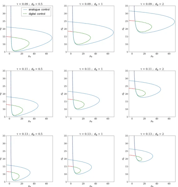
Fig. 2. Stability charts for different values ofτ anddψ. Blue lines indicates the D-curves for the analogue control. Red and green lines indicates the transition curves of the digital control.
where Q(t) is the control torque acting between the reaction wheel and the body of the pendulum. A PD control is assumed for ϕ and a D controller for ψ. Two models are distinguished. In case of analogue control with feedback delay,
Q(t) =Pϕϕ(t−τ) +Dϕϕ(t˙ −τ) +Dψψ(t˙ −τ). (3) Here, the control torque is updated continuously with feedback delayτ. In case of digital controller, the sampling effect is modeled as a zero order hold. Thus, the control torque is kept constant over the sampling interval t ∈ [ti, ti+1) as
Q(t) =Pϕϕ(ti−τ) +Dϕϕ(t˙ i−τ) +Dψψ(t˙ i−τ), (4) where ti =iτ denotes the sampling instants. Introducing the new parameters
a= g(L m+l md) l2md+JA
, k= l2md+JA Jd
(5) pϕ= Pϕ
l2md+JA
, dϕ= Dϕ
l2md+JA
(6) dψ= Dψ
l2md+JA (7)
the governing equations can be rewritten as
¨
ϕ(t)−α2ϕ(t) =−pϕϕ−dϕϕ˙−dψψ,˙ (8) ψ(t) =¨ kpϕϕ+kdϕϕ˙+kdψψ.˙ (9) 2.1 Stability in case of analogue control
In case of analogue control, first-order representation of the system is
x(t)˙ −A x(t)−B D x(t−τ) = 0, (10) where
A=
0 1 0 α2 0 0 0 0 0
, D=
"−pϕ
−dϕ
−dψ
#T
, B=
" 0 1
−k
# . (11) The corresponding characteristic equation reads
D(λ) =α2dψk e−λτ+λ pϕe−λτ−α2
+λ2e−λτ(dϕ−dψk) +λ3 (12) The D-curves, where the system has characteristic roots at the imaginary acces can be given as
pϕ(ω) = (α2+ω2) cos(τ ω), (13) dϕ(ω) = (α2+ω2)(dψk+ωsin(τ ω))
ω2 . (14)
The stability diagrams can be seen in the Fig. 2. The stable regions are the ones within the loops of the blue curves. The corresponding parameters are l = 0.3 m, L = 0.2015 m, JA = 0.033 kgm2, Jd = 0.0044546 kgm2, m = 0.64 kg, md = 0.23 kg. These parameters were determined for the experimental realization of the system (see Section 3).
2.2 Stability in case of digital control
In case of digital control, first-order representation of the system is
˙
x(t) =A x(t) +BD x(ti−τ), t∈[ti, ti+1), (15) where ti = iτ, i = 1,2, . . . are the sampling instants.
Solving the system over a sampling interval gives the discrete map
xi+1
ui
= P R
D 0
| {z }
:=G
xi
ui−1
(16)
where
P=eAτ, R=
τ
Z
0
eA(τ−s)B (17) The coefficient matrixGcan be derived as
G=
cosh(ατ) sinh(ατα ) 0 cosh(ατα2)−1
αsinh(ατ) cosh(ατ) 0 sinh(ατα )
0 0 1 −kτ
−pϕ −dϕ −dψ 0
(18)
The system is stable if all the eigenvalues of matrix G are in magnitude less than 1. The corresponding stability diagrams are shown in Fig. 2. The stable regions are the ones within the loops of the green curves.
Fig. 3. Realization of an inverted pendulum controlled by reaction wheels
3. EXPERIMENTAL BALANCING DEVICE The realized inverted pendulum under study is shown in Fig. 3. The body of the pendulum is a plastic U-profile, which carries a 9.6 V battery. The reaction wheel attached to the top of the pendulum consists of three spokes with masses at the end. The wheel is driven by a brushed DC motor equipped with a two-channel Hall encoder. The control is performed by an Arduino Uno microcontroller. A six-axis gyro- and accelerometer is attached to the body of the pendulum. The angular position and the angular velocity of the pendulum is determined using the hori- zontal (xdirection) and vertical (y direction) acceleration and the angular velocity along the pivot axis (zdirection).
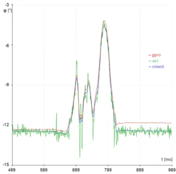
The accelerometer can be used to measure approximately the deviation from the gravitational acceleration, hence from vertical. The integral of the gyro signal also gives an estimation of the angular position. This signals from the accelerometer and the gyro are combined with the integral of the gyro signal. The different signals and their combination can be seen in Fig. 4.
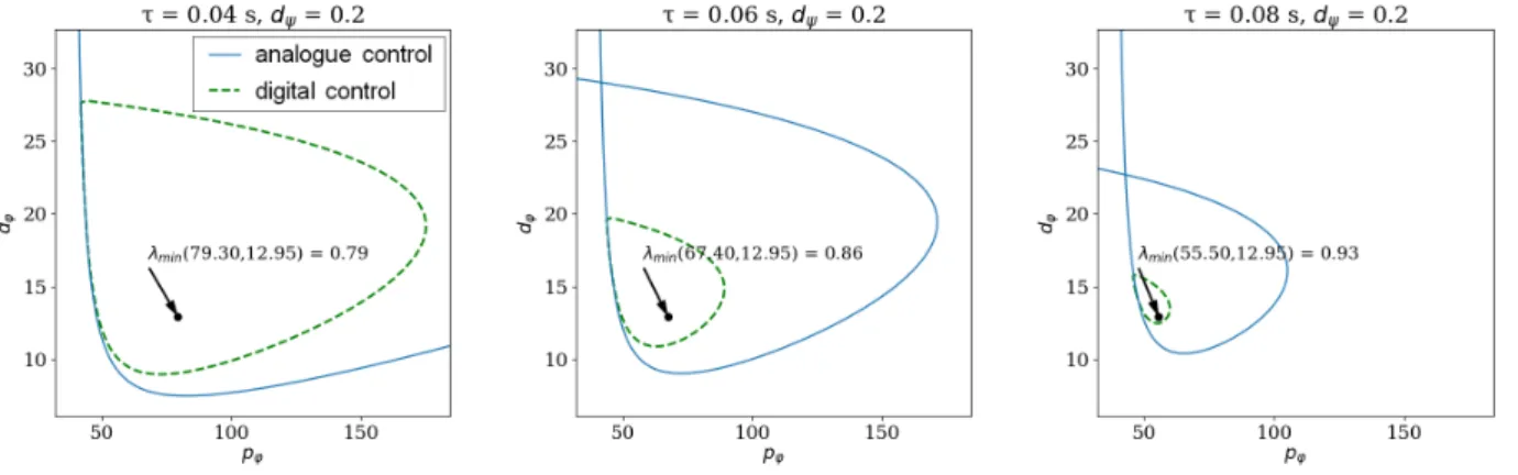
For the experiments, the feedback delay and the control gains were set to τ = 0.04 s, pϕ = 79.3, dϕ = 12.96, dψ = 0.2, respectively. Figures 5 and 6 show some sta- bility diagrams associated with the experimental device for different values of sampling periodτ and control gain dψ. It can be seen that the selected parameter point is robust to both in the changes in sampling period τ and the control gainspϕ,dϕanddψ. Thus, it is expected that the pendulum is easily balanced for these parameters.
The time history of the experimental device for this pa- rameters are shown in Fig. 7. The computed control torque (Qtheo) and the real one (Qreal) determined by inverse dy- namics show good agreement. This indicates that the effect of the so-called unmodeled dynamics is modest. It can be seen that pendulum is stabilized about its upper equilib-
Fig. 4. Angular position signal obtained by the integral of the gyro signal (red), by the accelerometer only (green) and their combination (blue).
Fig. 5. Stability diagrams for the experimental device in case of fixeddψ= 0.2.
Fig. 6. Stability diagrams for the experimental device in case of fixedτ = 0.04 s.
Fig. 7. Time series for a balancing test. Stability is lost att= 27 s.
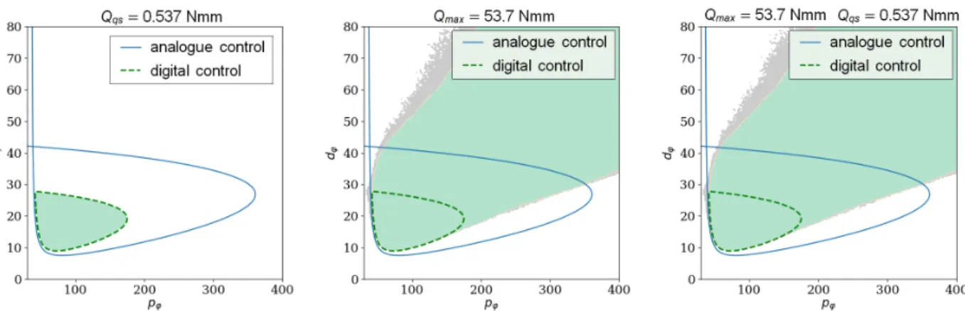
Fig. 8. Stability diagram in case of quantized control torque (left), in case of saturated control torque (middle) and in case of quantized and saturated control torque (right).
Fig. 9. Simulated time history in case of transient stabilization.
rium with some small fluctuations, then after 27 s, it falls.
The explanation for this transient behavior might be the slow changes in the system parameters during operation.
Another explanation can be the occurrence of transient chaos, which is a typical phenomenon in digitally controller machines (Lai and Tel, 2011; Csernak and Stepan, 2005).
In order to analyze the behavior of the system, the model is extended with nonlinear terms, namely, saturation and the quantization of the control torque.
4. TORQUE SATURATION AND QUANTIZATION Quantization and saturation of the control torque repre- sent a strong nonlinearity in the governing equations. The realized control torque can be written as
Qrealized(t) =
Qquant(t) if|Qquant(t)|< Qmax Qmax if|Qquant(t)| ≤Qmax
, (19) where
Qquant(t) =QqsInt
Qcom(t) Qqs
(20) is the quantized control torque with Int being the integer part function (rounds towards zero). Here, Qqs is the quantization step and
Qcom(t) =Pϕϕ(ti−τ) +Dϕϕ(t˙ i−τ) +Dψψ(t˙ i−τ), (21) is the commanded control torque in the sampling period t∈[ti, ti+1),ti=iτ.
The effect of quantization and saturation was investigated using numerical simulations. The parameter plane (pϕ, dϕ) was divided into 200×200 grid points for fixed dψ = 0.2 and τ = 0.04 s values. The system was declared to be stable if the simulated angleϕdoes not get larger in mag- nitude than 20◦. The results are shown in Fig. 8. Control gains, where the system experiences bounded oscillations are indicated by green shading. For comparison, linear stability boundaries of the digital controller are shown by green lines. It can be seen that quantization of step Qqs = 0.537 Nnm does not affect the local behavior of the system. Saturation at Qmax = 53.7 Nmm on the other hand significantly extends the region of control gains associated with bounded oscillations.
Numerical simulations showed that for certain control gains, the system is stabilized only for certain time period.
These parameter regions are indicated by grey shading in Fig. 8. This is similar to the experimentally observed transient stabilization. A sample time history is shown in Fig. 9, where stabilization (i.e., bounded motions about the upper equilibrium) was achieved only for 90 seconds.
5. CONCLUSIONS
An experimental device was built to demonstrate tran- sient behavior of digitally controlled machines. The main components of the underlying dynamics are the digital
sampling, signal quantization and actuation saturation.
The experimental system showed transient stabilization for certain control gain parameters. This phenomenon was shown to exist in the mechanical model of the system, too. Systematic numerical simulation demonstrated that slight quantization of the control torque did not signifi- cantly change the local behavior of the system. On the other hand, saturation of the control torque was shown to essentially increase the region of stability in the plane of the control gains.
In addition to the significance for robot control, the phe- nomenon of transient stabilization has significant conse- quences to human motor control. Many human activities can be associated with a similar feedback mechanism, for instance, simple quiet standing, gait, running or other balancing tasks like stick balancing on the fingertip. The corresponding models are all related to the stabilization of an inverted pendulum (Cabrera and Milton, 2002; Mehta and Schaal, 2002; Maurer and Peterka, 2005; Milton et al., 2009; Suzuki et al., 2012). Similarly to robot control, human motor control involves a reaction delay (dead time), sensory uncertainties (quantization) and saturation at some level of the control torque. Therefore experiments with inverted pendulums (Qin et al., 2014; Xu et al., 2017; Kovacs and Insperger, 2018), where the effect of the change of these parameters can be investigated, are of key importance for human balancing research, too.
ACKNOWLEDGEMENTS
The research reported in this paper was supported by the Higher Education Excellence Program of the Ministry of Human Capacities in the frame of Artificial intelligence research area of Budapest University of Technology and Economics (BME FIKP-MI).
REFERENCES
Cabrera, J.L. and Milton, J.G. (2002). On-off intermit- tency in a human balancing task. Physical Review Letters, 89, 158702.
Csernak, G. and Stepan, G. (2005). Life expectancy of transient microchaotic behavior. Journal of Nonlinear Science, 15, 63–91.
Delchamps, D.F. (1990). Stabilizing a linear system with quantized state feedback. IEEE Transactions on Automatic Control, 35(8), 916–924.
Erneux, T. and Kalmar-Nagy, T. (2007). Nonlinear sta- bility of a delayed feedback controlled container crane.
Journal of Vibration and Control, 13(5), 603–616.
Gajamohan, M., Muehlebach, M., Widmer, T., and D´Andrea, R. (2013). The Cubli: a reaction wheel based 3D inverted pendulum. InEuropean Control Conference (ECC), 268.
Gorinevsky, D.M., Formalsky, A.M., and Schneider, A.Y.
(1997). Force control of robotics systems. CRC Press, Boca Raton, FL.
Habib, G., Miklos, A., Enikov, E. T. an Stepan, G., and Rega, G. (2017). Nonlinear model-based parameter estimation and stability analysis of an aeropendulum subject to digital delayed control. International Journal of Dynamics and Control, 5(3), 629–643.
Hu, H.Y. and Wang, Z.H. (2002). Dynamics of controlled mechanical systems with delayed feedback. Springer, Heidelberg.
Kovacs, B.A. and Insperger, T. (2018). Retarded, neutral and advanced differential equation models for balancing using an accelerometer. International Journal of Dy- namics and Control, 6(3), 982–989.
Lai, Y.C. and Tel, T. (2011). Transient chaos: Complex dynamics on finite time scales. Springer, New York.
Lehotzky, D., Insperger, T., and Stepan, G. (2018). Nu- merical methods for the stability of time-periodic hybrid time-delay systems with applications. Applied Mathe- matical Modelling, 57, 142–162.
Maurer, C. and Peterka, R.J. (2005). A new interpretation of spontaneous sway measures based on a simple model of human postural control. Journal of Neurophysiology, 93, 189–200.
Mehta, B. and Schaal, S. (2002). Forward models in visuomotor control. Journal of Neurophysiology, 88, 942–953.
Milton, J.G., Ohira, T., Cabrera, J.L., Fraiser, R., Gyorffy, J., Ruiz, F.K., Strauss, M.A., Balch, E., Marin, P., and Alexander, J.L. (2009). Balancing with vibration: a prelude for “drift and act” balance control. PLoS One, 20(10), e7427.
M¨uhlebach, M. and D´Andrea, R. (2017). Nonlinear anal- ysis and control of a reaction-wheel-based 3-D inverted pendulum. IEEE Transactions on Control Systems Technology, 25(1), 235–246.
Munoa, J., Mancisidor, I., Loix, N., Uriarte, L.G., Barcena, R., and Zatarain, M. (2013). Chatter suppression in ram type travelling column milling machines using a biaxial inertial actuator. CIRP Annals, 62(1), 407–410.
Otto, A., Radons, G., Bachrathy, D., and Orosz, G.
(2018). Synchronization in networks with heterogeneous coupling delays. Physical Review E, 97(1), 012311.
Qin, Z.C., X., L., Zhong, S., and Sun, J.Q. (2014). Control experiments on time-delayed dynamical systems. Jour- nal of Vibration and Control, 20(6), 827–837.
Stepan, G. (2001). Vibrations of machines subjected to digital force control.International Journal of Solids and Structures, 38(10-13), 2149–2159.
Stepan, G., Milton, J.G., and Insperger, T. (2017). Quanti- zation improves stabilization of dynamical systems with delayed feedback. Chaos, 27(11), 114306.
Suzuki, Y., Nomura, T., Casadio, M., and Morasso, P.
(2012). Intermittent control with ankle, hip, and mixed strategies during quiet standing: A theoretical proposal based on a double inverted pendulum model. Journal of Theoretical Biology, 310, 55–79.
Ushio, T. and Hsu, C. (1987). Chaotic rounding error in digital control systems. IEEE Transactions on Circuits and Systems, 34(2), 133–139.
Xu, Q., Stepan, G., and Wang, Z. (2017). Balancing a wheeled inverted pendulum with a single accelerometer in the presence of time delay. Journal of Vibration and Control, 23(4), 604–614.
Zhang, L., Sun, J., and Orosz., G. (2018). Hierarchical design of connected cruise control in the presence of in- formation delays and uncertain vehicle dynamics.IEEE Transactions on Control Systems Technology, 26(1), 139–150.