Control of Tumor Growth by Modern Control Methodologies
Gy¨orgy Eigner
Physiological Controls Research Center Research and Innovation Center Obuda University, Budapest, Hungary´ Email: eigner.gyorgy@nik.uni-obuda.hu
Levente Kov´acs
Physiological Controls Research Center Research and Innovation Center Obuda University, Budapest, Hungary´ Email: kovacs.levente@nik.uni-obuda.hu
Abstract—The role of modern control engineering in physi- ological controls cannot be questioned. However, practitioners have to face with many challenges in the field. The imprecise information of the state variables of the system to be controlled, significant inter- and intra-patient variability, limitations regard to the applied sampling frequency are just a few of them. The current study investigates a possible solution for those issues related to control of tumor growth. In order to describe the parameter variabilities Linear Parameter Varying (LPV) method has been used and extended by applying Tensor Product (TP) model transformation. We formulated the goals of the control by using Linear Matrix Inequalities (LMI). Parallel Distributed Control can be used based on the state-feedback gains obtained through LMI optimization. The unmeasurable states can be estimated by using Extended Kalman Filtering. By using these techniques we were able to realize a control framework which enforces our original nonlinear system to behave as a given reference system within limitations. We have found that the developed control framework operates satisfactory by reaching all of the determined goals of the control.
Index Terms—Tensor Model transformation, Linear Parameter Varying, Linear Matrix Inequality, Parallel Distribution Control, tumor control
I. INTRODUCTION
Targeted Molecular Therapies (TMTs) are one of those innovative therapeutic proceedings which directly inhibit or eliminate specific properties of given kind of cancers [1]. They have many advantages, e.g. more specific targeting, the use of less aggressive chemicals, more limited side effects than regular therapies (like radiotherapy and chemotherapy) [1], [2].
One of the well known attribution of all kind of tumors is that they are not able to reach higher volume than a certain level by exploiting only the diffusion for nutrient intake. In order to fight down this barrier tumor cells producing angio- gen factor, the so-called vascular endothelial growth factor (VEGF). VEGF catalyzes the endothelial cell proliferation which leads to the formation of new blood vessels – these become the main source of nutrients beyond the distance of
Gy. Eigner was supported by the ´UNKP-17-4-I. New National Excellence Program of the Ministry of Human Capacities. This project has received funding from the European Research Council (ERC) under the European Union’s Horizon 2020 research and innovation programme (grant agreement No 679681)
diffusion [3]. By inhibiting this phenomena, namely, by hinting the formation of the supporting vasculature, the size of the tumor can be kept or decreased under a given level. This antiangiogen treatment can be done by TMTs as well, where one of the most applied drug is bevacizumab [4].
As a result, from control engineering point of view the ther- apy can be described as a control problem in which the goal is to determine the amount of injectable drug automatically.
There have been efforts to investigate this control problem in the last decade [2], [5]–[8]. However, many issues – similarly to other physiological control directions – are still unsolved, for example, the effective handling of nonlinearities, parameter uncertainties and variabilities and so on.
The Linear Parameter Varying (LPV) framework is able to deal with the mentioned challenges effectively. By enclosing the nonlinearity causing terms of the applied mathematical model into a given parameter vector the use of linear controller design techniques is possible. The polytopic LPV approach (considered in this study as well) allows to design particpular controllers only to the extremes of the parameter vector which are connected via common weighting functions [9], [10]. LPV methods can be alloyed with Tensor Product (TP) model transformation which makes possible to describe the LPV
”function” as a convex combination of different subsystems [11], [12]. The TP model transformation can be connected to Linear Matrix Inequality (LMI) based controller design as well. LMIs are powerful tools which allows us to formulate the control problems and constraints coming from the system to be controlled as optimization problems [13].
The paper proposes to apply such a control strategy for antiangiogenic tumor treatment and is structured in the follow- ing way. First, the applied tumor growth and LPV models are introduced. After, the controller design is detailed including the TP model transformation, applied LMIs and Extended Kalman Filter (EKF) design. Finally, we conclude our work and introduce our future plans regarding the research.
II. INVESTIGATEDMODELS
A. The Minimal Tumor Growth Model
The minimal tumor growth model was introduced in [14], [15]. The model operates with two state variables which
978-1-5386-2203-2/18/$31.002018c IEEE
describe the volume of the tumor and the inhibitor serum level, respectively. The model can be described by the following differential equations:
˙
x1(t) =ax1(t)−bx1(t)x2(t)
˙
x2(t) =−cx2(t) +u(t) , (1) where x1(t) [mm3] is the volume of the tumor and x2(t) [mg/kg] is the inhibitor serum level. The input of the model is the inhibitor intakeu(t)[mg/kg/day]. The output of the model is its first state, the tumor volume x1(t), which is assumed to be measurable.
The model has three scalar parameters: tumor growth rate a [1/day], inhibitor rate b [kg/mg/day] and inhibitor clear- ance c [1/day], respectively. In this study we have used the following parameter set during our investigations: a = 0.27 [1/day], b = 0.0074 kg/mg/day and c = ln(2)/3.9 [1/day].
These parameters are considered as belonging to a ”virtual patient” related to treatment by bevazicumab (the numerical values coming from parametric identification based on mice experiments regard to C38 colon adenocarcinoma) [14].
The model is a mathematical description of the phenomena and assumes that the tumor volume can be decreased by using antiangiogen inhibitor – represented by u(t). Although, it is composed by only two state variables, the handling of the model is challenging due to it’s unstable nature. Without any inhibitionx1(t)grows limitlessly determined by theagrowing factor. The model’s nontrivial equilibrium can be determined by solving the following equation:
0 =ax1,∞−bx1,∞x2,∞
0 =−cx2,∞+u∞ , (2)
which indicates that the x2,∞ = a/b and u∞ = c·a/b are independent from x1,∞. This means, in accordance with the model parameters x2,∞ = a/b is needed in order to keep a constant tumor volume belonging tou∞=c·a/b. If the goal is to decrease the tumor volume, we have to apply a higher inhibitor level than this certain level.
These properties are model specificities, which have to be taken into account during the controller design.
B. Applied qLPV Models
An LPV model can be represented in state-space form as follows [9], [16]:
˙
x(t) =A(p(t))x(t) +B(p(t))u(t) y(t) =C(p(t))x(t) +D(p(t))u(t)
x(t)˙ y(t)
=S(p(t)) x(t)
u(t)
S(p(t)) =
A(p(t)) B(p(t)) C(p(t)) D(p(t))
, (3)
where x(t) ∈ Rn, y(t) ∈ Rk, u(t) ∈ Rm are the state-, output- and input-vectors, respectively. The A(t)∈ Rn×n is the state matrix, B(t) ∈ Rn×m is the control input matrix, C(t) ∈ Rk×n is the output matrix, D(t) ∈ Rk×m is the control feed-forward matrix. p(t) = [p1(t). . . pR(t)] is the parameter vector which is built up from scheduling parameters
pi(t). The p(t)∈ΩR∈RR is anR dimensional real vector within the Ω = [p1,min, p1,max]×[p2,min, p2,max]×. . .× [pR,min, pR,max]∈ RR hypercube inside the RR real vector space. The S(p(t)) ∈ R(n+k)×(n+m) is the system matrix, which is an LPV function at the same time. If any of the states is selected as scheduling variable, the given LPV model becomes a quasi-LPV (qLPV) model [9].
Assume that the nonlinearity causing terms of a given, nonlinear model are selected as scheduling variablespi(t). In this case we can encapsulate the nonlinearity into thep(t)and we are able to use linear control methodologies on the LPV construct – in this way, on the original model as well.
It should be noted that we have applied two different LPV models. Thus, we denoted their parameter vectors asq(t)∈R1 andp(t)∈R2, respectively.
1) Model-A: By selecting q(t) = x1(t) as scheduling variable the following LPV model occurs from (1):
˙
x(t) =AA(q(t))x(t) +BAu(t) y(t) =CAx(t)
SA(q(t)) =
AA(q(t)) BA
CA 0
=
a −bq(t) 0
0 −c 1
1 0 0
, (4)
where q(t) ∈ {10−3, . . . ,5 ×105}, BA = B and CA = C. The lower border is the approximation of the zero level.
The A subscript relates to Model-A. This is physiologically meaningful, since, the goal of TMT therapies – in general – is the inhibition of the tumor and not to eliminate it. Moreover, this is beneficial to keep the numerical stability of the system as well. The upper boundary is in accordance with previous investigations [17]. Model-A has been used for the Extended Kalman Filter design as it will be presented in the latter part of the study.
2) Model-B: For the controller design we have developed a difference based control oriented qLPV model. This construct is beneficial for state-feedback controls. By applying this method the reference compensation – which is needed for state-feedback with nonzero reference – becomes unnecessary.
We model the error dynamics, namely, the deviation of the system from a certain reference system. Thus, we have applied the following transformed states:∆x1(t) =x1(t)−x1,ref(t),
∆x2(t) = x2(t)−x2,ref(t) and ∆u(t) = u(t)−uref(t) instead of the states from (1). These new states characterize the ”error dynamics” and allow the use of zeror=02×1 ref- erence. Therefore, the control goal becomes to reach the zero level by the ∆x(t) = [x1(t), x2(t)]>, namely, ∆x(t) → 0, while t → ∞. The transformation of the states can be done
in the following way:
∆ ˙x1(t) = ˙x1(t)−x˙1,ref(t) = ax1(t)−bx1(t)x2(t)
− ax1,ref(t)−bx1,ref(t)x2,ref(t)
= a∆x1(t)−bx1(t)x2(t)−bx1,ref(t)x2,ref(t) + 0 =
a∆x1(t)−bx1(t)x2(t)−bx1,ref(t)x2,ref(t) +bx1(t)x2,ref(t)−bx1(t)x2,ref(t) = (a−bx2,ref(t))∆x1(t)−bx1(t)∆x2(t)
∆ ˙x2(t) = ˙x2(t)−x˙2,ref(t) =
−cx2(t) +u(t)− −cx2(t) +u(t)
=
−c∆x2(t) + ∆u(t)
. (5)
The qLPV model can be represented in state-space form as follows:
∆ ˙x(t) =AB(p(t))∆x(t) +BB∆u(t)
∆y(t) =CB∆x(t) SB(p(t)) =
AB(p(t)) BB
CB 0
=
a−bp1(t) −bp2(t) 0
0 −c 1
1 0 0
, (6)
where the selected scheduling variables became p1(t) = x2,ref(t) ∈ {a/b+ 10−3, . . . ,104} and p2(t) = x1(t) ∈ {10−3, . . . ,5 ×105} – with p(t) = [p1(t), p2(t)]>. The p1,min = x2,ref,min = a/b+ 10−3 which is necessary to keep the controllability of Model-B. This is coming from the property of the original model (1): the serum inhibitor level has to be higher than a/b[mg/kg] in order to decrease the tumor volume x1(t) over time. By applying a/b+ 10−3 this can be approached. The p1,max was selected as the physiologically highest value which was considered regard to previous investigations [17]. The extremes ofp2(t)is the same as q(t).
III. CONTROLLERDESIGN
A. Tensor Product Model Transformation and Control The TP model transformation allows to represent a given qLPV function from (3) as finite element convex polytopic TP model in the following way:
x(t)˙ y(t)
=S(p(t)) x(t)
u(t)
S(p(t)) =S R
r=1wr(pr(t)) =S ×rw(p(t))
, (7)
where S ∈ RI1×I2×...×IR×(n+k)×(n+m) core tensor contains Si1,i2,...,iR linear time invariant (LTI) systems as vertices. The wr(pr(t))weighting vector built up from wr,ir(pr(t)) (ir= 1...IR)continuous convex weighting functions. The convexity is satisfied, if∀r, i, pr(t) :wr,ir(pr(t))∈[0,1]and∀r, pr(t) :
Ir
X
i=1
wr,ir(pr(t)) = 1. Several convex hull types can be used.
We have applied the Minimal Volume Simplex (MVS) kind convex hull in this work [11].
The realization steps of the TP model transformation can be found in [11], [12], [18].
A general LPV controller based on state-feedback can be realized in the following way:
u(t) =r(t)−G(p(t))x(t) , (8) where G(p(t)) ∈ Rm×n is the parameter dependent con- troller gain. If r(t) = 0n×1, then (8) simplifies to u(t) =
−G(p(t))x(t). A TP based state-feedback controller in poly- topic structure can be described as follows:
G(p(t)) =Gr=1R wr(pr(t)) =G ×rw(p(t)) . (9) Here G is the feedback tensor which contains Gi1,i2,...,iR
feedback gain matrices – as vertices – belong to the given Si1,i2,...,iRLTI systems andwr(pr(t))is the same as in (7). In this way, the resulting feedback gainG(p(t))can be described as the convex combination of the gains in the vertices.
B. Linear Matrix Inequality based Optimization
In polytopic case and in accordance with Lyapunov’s direct method, the system equation is
˙
x(t) = A(p(t))x(t) + B(p(t))u(t) and the polytopic vertices are [A(p(t)) B(p(t))] =
R
X
r=1
wr(p)[Ar Br], where wr(p)is a general, convex polytopic weighting function [12].
By considering theV(x(t)) =x>Px=x>X−1x Lyapunov function, the possible controller candidate can be written as:
u(t) =M(p(t))X−1x(t) =
J
X
j=1
wj(p)MjX−1x(t) . (10) The derivative of the Lyapunov function becomes as follows:
V˙(x(t)) =
x>(t)X−1·Sym A(p)X+B(p)M(p)
X−1x>(t) , (11) where the acronym ”Sym” means symmetric term – which can be described by general polytopic weighting functions as:
Sym A(p)X+B(p)M(p)
=
R
X
i=1 R
X
j=1
wi(p)wj(p)Sym AiX+BiMj
≺0 . (12) In respect to this given case, the S(p(t)) = Co(S1,S2, . . . ,SR) and K(p(t)) = Co(G1,G2, . . . ,GR) are polytopic structures (the ”Co” means convex combination).
Due to the applied samew(p(t))convex weighting functions, the Parallel Distributed Compensation (PDC) kind control can be realized [12], [19].
A quadratically stabilizing PDC for continuous polytopic system can be designed by LMI optimization:
X0,
−XA>i −AiX+M>i B>i +BiMi0,
−XA>i −AiX−XA>j −AjX +M>jB>i +BiMj+M>i B>j +BjMi0, i < j ≤R s.t. ∀p(t) :wi(p(t))wj(p(t)) = 0
. (13)
HereXn×nsymmetric, positive definite matrix,Mm×ni is the complementary matrix and wi and wj are general polytopic weighting functions. The control gain can be calculated by Mi=GiX, thus,Gi =MiX−1 [19].
Due to the amount of injectable inhibitor is limited, we have applied input limitation as well to avoid the unrealistically high dosage from the drug. This property can be handled by given LMI constraint on the control input which guarantees that ku(t)k2≤µatt≥0. This property holds for polytopic cases, ifx(0)lies on the polytope, which requires thatkx(t0)k2≤1.
This can be extended for a minimization problem onµwhich requires the kV(x(t0))k2 ≤ 1. The necessary conditions during the LMI optimization are the followings [13]:
min
X,Mµ XI, X M>
M µ2I
0
. (14)
The LMI optimization can be merged with the TP model transformation. During the procedure we have used the Model- B from (6).
Due to the applied extremes of p(t) ∈
{pmin, . . . ,pmax} the rank of the controllability matrix rank(C(AB(p(t)),BB)) = n = 2 ∀p(t), namely, the Model-B is controllable on the whole Ω parameter domain.
By using these LMIs we have reached stable control in Lyapunov sense – completed by control input limitation.
C. Extended Kalman Filter Design
Due to the nature of the controlled phenomena we have applied a mixed continuous/discrete EKF [20] – the physio- logical system to be controlled operates in continuous time, however, the state estimation is happening via digital proces- sors. It should be noted, that we have used the Model-A for the Extended Kalman Filter (EKF) design and we realized an LPV-based EKF; the assumed sampling time was T = 1day – in accordance with the model properties.
The steps of the EKF design were the followings in this given case:
˙
x(t) =f(x(t),u(t)) +w(t), w(t)∼ N(0,Q(t)) yk=h(xk) +vk, vk∼ N(0,Rk) , (15) wherexk =x(tk)andf =AA(p(t))x(t)+BAu(t)from (4).
The w(t) andvk is the system’s disturbance and the actual noise, respectively. The appliedhwas h=CAxk+vk – the discretization didn’t change the structure of the output from (4).
In accordance with the model properties we have considered that there is no additive noise and disturbance, namely,Q(t) = 0n×n and Rk = 0 (we have only one output). In the given circumstances, the EKF simplifies to an optimal estimator [20].
The xˆ0|0 = E x(t0)
and P0|0 = Var x(t0)
have been used as initial conditions, respectively.
In the prediction phase, the following differential equations have to be solved with respect to x(tˆ k−1) = ˆxk−1|k−1 and P(tk−1) =Pk−1|k−1:
˙ˆ
x(t) =f(ˆx(t),u(t))
P(t) =˙ F(t)P(t) +P(t)F>(t) +Q(t) , (16) whereF(t) = ∂f
∂x ˆx,u
. The solution is needed for the update phase asxˆk|k−1= ˆx(tk)andPk|k−1=P(tk).
The first step of the update phase is the update of the Kalman gain:
Kk =Pk|k−1H>k(HkPk|k−1H>k +Rk)−1 , (17) whereHk = ∂h
∂x ˆx
k|k−1
.
In the second step of the update phase the following difference equation has to be solved:
ˆ
xk|k= ˆxk|k−1+Kk(yk−h xˆk|k−1))
Pk|k = (I−KkHk)Pk|k−1 , (18) whereIis the identity matrix in appropriate dimensions.
D. Final Control Structure
Figure 1. Structure of the control loop.
During the design, the original model was considered the reference model – however, without any uncertainty. Naturally, this model can be replaced by other beneficially selected reference models.
The final control structure can be seen on Fig. 1. We have used permanent uref(t) = uref, which was able to provide appropriate trajectory for thexref(t)states. During the uref
calculation, two constraints have been considered. The first constraint was to preserve the controllability of Model-B, which requires the application of uref > c·(a/b+ 10−3) due to the model properties. This action guarantees that x2,ref =p1≥a/b+ 10−3, since, the original model plays the role of the reference system as well. Our goal was thatx1<1 [mm3] within the simulated treatment period – which has been taken into account as second constraint. The belonging uref was calculated in this form: uref = c · (a/b+d), wheredguarantees the x1,ref <1 [mm3] – which leads that
x1(tf inal)<1due to the control framework. The structure of the uref calculation was selected arbitrarily, since, only the addition of an affine term was necessary somewhere into the equation.
The designed controller enforces the states of the original nonlinear model to behave as the selected reference model over time. Thus, x(t) =xref(t),t→ ∞, which is equivalent to∆r=x−xref =0.
Due to the EKF is an optimal estimator now and we are not able to measurex2(t)directly, thex(t)ˆ has been used instead of x(t)during the error signal generation. Therefore, ˆx(t)− xref(t) was compared to ∆r =0by the control framework and it acted in accordance with the control law.
IV. RESULTS
From the realization point of view two important aspects are needed to be emphasized. The first is that during the realization we have used the Euler’s forward method, namely, dx(t0)/dt≈(x(t0+T)−x(t0))/T, whereT is the sampling time. Secondly, we have used MATLAB environment during the development. As we mentioned, we did not consider dis-
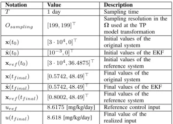
Table I
DETERMINING VALUES OF THE NUMERICAL SIMULATION.
Notation Value Description
T 1day Sampling time
Osampling [199,199]>
Sampling resolution in the Ωused at the TP model transformation x(t0) [3·104,0]> Initial values of the
original system ˆ
x(t0) [10−3,0]> Initial values of the EKF xref(t0) [3·104,36.4875]> Initial values of the
reference system x(tf inal) [0.5742,48.49]> Final values of the
original system ˆ
x(tf inal) [0.5742,48.49]> Final values of the EKF xref(tf inal) [0.8002,48.49]> Final values of the
reference system uref 8.6175[mg/kg/day] Reference control input u(tf inal) 8.618[mg/kg/day] Final value of the
realized input
turbances and noises in accordance with the model properties – which has to be taken into account the design of the EKF.
Thus, we appliedd≡0 andn≡0 during the examination.
Table I. contains all the considered constraints, initial con- ditions and final values.
We assumed that x1(t0) is known at beginning of the treatment and x2(t0) = 0 – which represents that there is no inhibitor in the blood before the therapy.
The initial states of the EKF are significantly different than the other initial values; in this way the operation of it is clearly visible. The initial states of the reference model are coming from two facts: the tumor volume has to be x1(t0) =x1,ref(t0)(for the accurate therapy) andx2,ref(t0) is x2,ref(t0)≥a/b+ 10−3 due to the reasons connected to uref > c· (a/b+ 10−3). Figure 2. shows the trajectories of the states of the original system, EKF and reference models, respectively. As we mentioned, the EKF approaches
0 20 40 60 80 100
0 2 4 104
0 50 100
0 20 40 60 80 100
0 2 4 104
0 50 100
0 20 40 60 80 100
0 1 2 3
104
0 20 40
Figure 2. Trajectories of the state variables.
0 20 40 60 80 100 120
0 1 2 3 104
-1 -0.5 0 0.5 1
0 20 40 60 80 100 120
-1 0 1 2 3 104
-100 -50 0 50
Figure 3. Deviations between the states of the models.
the original model with high precision. Both thex(t)andx(t)ˆ approach thexref(t). Due to the EKF behaves as an optimal estimator,x(t)≈x(t),ˆ t >1.
The goal of the control – x1(tf inal) < 1 [mm3] – has been satisfied, since x1(tf inal) = 0.5742 [mm3]. Figure 3.
represents the deviations between the states of the models – the so-called state errors. As we have already mentioned, there is only numerical difference after the first update period between thex(t)andx(t). Atˆ t0, the errorx(t)-x(t) = [∼ˆ 3·104,0]>
due to different initial values as it can be seen in Table I.
The xref(t)−ˆx(t) can be used to measure the deviation between the reference and original model as well, sincex(t)≈ ˆ
x(t),t >1.
It can be seen that the ˆx(t) approaches the xref(t) over time. At tf inal the deviation between x1,ref(tf inal) and ˆ
x1,ref(tf inal)is0.226[mm3] and0in case of the second state – which also strengthen the validity of the control framework.
Figure 4. shows the reference and control input during the simulation, moreover, the difference between them. At
0 20 40 60 80 100 8.2
8.4 8.6 8.8 9
0 20 40 60 80 100
0 20 40 60 80
0 20 40 60 80 100
-60 -40 -20 0
Figure 4. The reference and realized control signals.
the beginning of the u(t) there is a higher peak which comes from the aforementioned initial state dissimilarity as a consequence of state-feedback control. The final deviation isuref(tf inal)−u(tf inal) = 5·10−4 [mg/kg/day], moreover, uref(t)−u(t)<0.1after t >19.
The level of the totally injectable inhibitor based on the ref- erence control signal was
120
X
t=0
uref(t)·T = 1.0341·103[mg/kg]
(due to the Euler method instead of numerical integration a simple sum can be used). On the other hand, the actual realized total inhibitor level used during the simulated therapy became
120
X
t=0
u(t)·T = 1.0683·103 [mg/kg] and 34.1787 [mg/kg]
obtains as discrepancy.
V. CONCLUSION ANDFUTUREWORK
We have designed a difference based qLPV model for control purposes. Model-B has been used during the TP model transformation to get it’s TP model form. We applied Lyapunov’s second law and control input limitation via LMIs for polytopic LPV systems during the controller design which has provided stable control in Lyapunov sense. In this way a TP-LPV-LMI controller was realized.
We have used the original model as reference system in this study to generate appropriate trajectories needed to be followed by the original nonlinear model. For that we have applied permanent reference control signal.
We examined the behavior of the developed control frame- work. Our results showed that the controller operated well and all of the control objectives have been performed – the original model has approached the reference system with good accuracy.
In our future work we will focus to the application of more sophisticated reference models which provide more suitable state trajectories for trajectory tracking purposes. In this study,
we have used a random – but reasonable – initial value for the initialization of EKF which leads high control signal at the beginning due to the bigger state discrepancies. We will investigate the possibility of applying ”better” initial values in order to reduce the high initial control actions, and will combine other control methods as well [21].
REFERENCES
[1] P. Charlton and J. Spicer, “Targeted therapy in cancer,”Medicine, vol. 44, no. 1, pp. 34–38, 2016.
[2] N. Vasudev and A. Reynolds, “Anti-angiogenic therapy for cancer: cur- rent progress, unresolved questions and future directions,”Angiogenesis, vol. 17, no. 3, pp. 471–494, 2014.
[3] R. Weinberg,The biology of cancer, 2nd ed. New York, USA: Garland Science, Taylor and Francis, 2014.
[4] A. M. Abdalla, L. Xiao, M. W. Ullah, M. Yu, C. Ouyang, and G. Yang,
“Current challenges of cancer anti-angiogenic therapy and the promise of nanotherapeutics,”Theranostics, vol. 8, no. 2, pp. 533–548, 2018.
[5] J. S´api, L. Kov´acs, D. Drexler, P. Kocsis, D. Ga´ari, and Z. S´api,
“Tumor volume estimation and quasi-continuous administration for most effective bevacizumab therapy,”PLoS ONE, vol. 10, no. 11, 2015.
[6] F. Lobato, V. Machado, and V. Steffen, “Determination of an optimal control strategy for drug administration in tumor treatment using multi- objective optimization differential evolution,”Comp Meth Prog Biomed, vol. 131, pp. 51–61, 2016.
[7] D. Drexler, J. S´api, and L. Kov´acs, “Potential Benefits of Discrete-Time Controller-based Treatments over Protocol-based Cancer Therapies,”
ACTA Pol Hung, vol. 14, no. 1, pp. 11–23, 2017.
[8] J. Klamka, H. Maurer, and A. Swierniak, “Local controllability and optimal control for amodel of combined anticancer therapy with control delays,”Math Biosci Eng, vol. 14, no. 1, pp. 195–216, 2017.
[9] A. White, G. Zhu, and J. Choi,Linear Parameter Varying Control for Engineering Applicaitons, 1st ed. London: Springer, 2013.
[10] L. Kov´acs, “Linear parameter varying (LPV) based robust control of type-I diabetes driven for real patient data,”Knowl-Based Syst, vol. 122, pp. 199–213, 2017.
[11] J. Kuti, P. Galambos, and P. Baranyi, “Minimal volume simplex (MVS) convex hull generation and manipulation methodology for TP model transformation,”Asian J Control, vol. 19, no. 1, pp. 289–301, 2017.
[12] P. Baranyi, Y. Yam, and P. Varlaki,Tensor Product Model Transfor- mation in Polytopic Model-Based Control, 1st ed. USA: CRC Press, 2013.
[13] S. Boyd, L. El Ghaoui, E. Feron, and V. Balakrishnan,Linear Matrix Inequalities in System and Control Theory. USA: SIAM, 1994, vol. 15.
[14] D. Drexler, J. S´api, and L. Kov´acs, “A minimal model of tumor growth with angiogenic inhibition using bevacizumab,” in 15th IEEE Inter- national Symposium on Applied Machine Intelligence and Informatics (SAMI 2017), Herl’any, Slovakia, pp. 185 – 190.
[15] D. Drexler, J. S´api, and L. Kov´acs, “Positive control of a minimal model of tumor growth with bevacizumab treatment,” in 12th IEEE Conference on Industrial Electronics and Applications (ICIEA), Siem Reap, Camabodia, 2017, pp. 2081–2084.
[16] O. Sename, P. G´asp´ar, and J. Bokor, “Robust control and linear param- eter varying approaches, application to vehicle dynamics,” ser. Lecture Notes in Control and Information Sciences. Springer-Verlag, 2013, vol.
437.
[17] J. S´api, “Controller-managed automated therapy and tumor growth model identification in the case of antiangiogenic therapy for most ef- fective, individualized treatment,” Ph.D. dissertation, ´Obuda University, Budapest, Hungary, 2015.
[18] P. Galambos and P. Baranyi, “TP model transformation: A systematic modelling framework to handle internal time delays in control systems,”
Asian J Control, vol. 17, no. 2, pp. 1 – 11, 2015.
[19] K. Tanaka and H. O. Wang,Fuzzy Control Systems Design and Analysis:
A Linear Matrix Inequality Approach, 1st ed. Chichester, UK: John Wiley and Sons, 2001.
[20] H. Musoff and P. Zarchan, Fundamentals of Kalman Filtering: A Practical Approach, 3rd ed. American Institute of Aeronautics and Astronautics, 2009.
[21] R. Precup, R. David, and E. Petriu, “Grey wolf optimizer algorithm- based tuning of fuzzy control systems with reduced parametric sensitiv- ity,”IEEE T Industr Electr, vol. 64, pp. 527 – 534, 2017.