Nullspace-based input reconfiguration architecture for over-actuated aerial vehicles
Tam´as P´eni and B´alint Vanek,Member, IEEE, Gy¨orgy Lipt´ak, Zolt´an Szab´o, Member, IEEE,J´ozsef Bokor, Fellow, IEEE
Abstract—A dynamic input reconfiguration architecture is pro- posed for over-actuated aerial vehicles to accommodate actuator failures. The method is based on the dynamic nullspace computed from the linear parameter-varying model of the plant dynamics.
If there is no uncertainty in the system, then any signal filtered through the nullspace has no effect on the plant outputs. This makes it possible to reconfigure the inputs without influencing the nominal control loop and thus the nominal control performance.
Since the input allocation mechanism is independent of the structure of the baseline controller, it can be applied even if the baseline controller is not available in analytic form. The applicability of the proposed algorithm is demonstrated via the case study of designing a fault tolerant controller for the Rockwell B-1 Lancer aircraft.
Index Terms—fault tolerant control, null space computation, linear parameter varying systems, control input reallocation, aircraft control
I. INTRODUCTION
T
HE most stringent requirements for improved reliability and environmental sustainability of safety critical flight control systems could only be satisfied with the most advanced fault tolerant control (FTC) techniques [1], [2]. The FTC system is required to detect and identify the failure and then to compensate its effect by reconfiguring the control system [3]. Focus on the environmental impact of the aircraft triggers the need for higher performance flight control systems, which leads to a paradigm shift from robust passive FTC towards active methods relying on switching, gain scheduled or linear parameter-varying (LPV) methods with certifiable algorithms [4]. In the past few years a wide variety of FTC design approaches have been proposed [5], [6].This paper focuses on the reconfiguration task in the case of actuator failures. The approach considered here is the control input reallocation, where the aim is to compensate the actuator failures by reconfiguring the remaining flight control surfaces such that the forces and moments required by the flight controller can be generated. A broad picture on the state- of-the-art control allocation methods can be found in [7]. One class of the several approaches developed so far is formed by
The authors are with the Systems and Control Lab, Institute for Computer Science and Control of Hungarian Academy of Sciences, H-1111, Kende u. 13-17, Budapest, Hungary. Corresponding author: Tam´as P´eni, e-mail:
peni.tamas@sztaki.mta.hu
The research leading to these results has received funding from the European Union’s Seventh Framework Programme (FP7/2007−2013) under grant agreement no. FP7-AAT-2012−314544. This paper was also supported by the J´anos Bolyai Research Scholarship of the Hungarian Academy of Sciences.
the nullspace (or kernel) based methods that can be applied if control input redundancy is available in the system [8]. As in aerospace applications this is often the case [9], this approach is a promising method for fault tolerant flight control design.
The classical kernel-based algorithms assume constant input direction matrices and thus use static matrix kernels [7], [8].
This concept is extended in [10] and [11] by using dynamic annihilators. Though the reconfiguration architecture in these papers is similar to that is proposed here, the algorithms in [10] and [11] highly depend on the linear time invariant (LTI) framework and thus their extension to the parameter varying case rises several theoretical problems. This paper proposes a different approach, which is promising for LPV applications as well.
The main component of the proposed reconfiguration ar- chitecture is the nullspace of the LPV system to be con- trolled. Although the nullspace of a dynamical system bears significant importance on several other fields of control as well [12],[13],[14] its numerical computation has been solved only partially so far. In [15] an algorithm based on matrix pencils is proposed to compute the dynamic kernel of an LTI system. Although this approach is computationally ef- ficient, it is based on frequency domain formulation, which prevents its extension to LPV systems. In [12] the nullspace of a parameter-dependent, memoryless matrix is addressed in connection with controller design. The paper uses linear- fractional representation (LFR), but it does not consider the case of dynamic kernels. Moreover, the method of [12] does not analyze and thus cannot guarantee the well-definedness of the kernel basis, which are also necessary to use the kernel in any further design process. The LFR-Toolbox [16] also provides a method for nullspace computation. The algorithm is similar to the one given in [12] and it can be applied for dynamical systems as well, but it does not work for the general case as it requires certain rank conditions to be satisfied. In this paper we revise the existing methods and assemble a complete tool for kernel computation that can be applied for parameter- dependent matrices and LTI/LPV dynamical systems as well.
The paper is structured as follows, Section II is devoted to the numerical computation of the parameter varying nullspace.
The proposed actuator reconfiguration architecture is discussed in Section III. The simulation example, using the B-1 aircraft is presented in Section IV, while the paper is concluded in Section V.
II. NULLSPACE COMPUTATION FOR PARAMETER-VARYING SYSTEMS
In this section the definition of the nullspace of a linear map is defined and the problem related to its numerical computation is addressed.
A. Nullspace of a linear map
Definition 1 (nullspace and its generator). Let L denote a linear map assigning to the elements of a linear input spaceU the elements of a linear output spaceY. The (right) nullspace (kernel) of L, denoted byN(L), is a subset (subspace) ofU that are mapped to 0, i.e. N(L) ={u∈ U | Lu= 0}. If for some linear map N : W → U, N(L) = Im(N), thenN is called the generatorof the nullspace.
The following lemma gives the basis of the nullspace construction algorithms derived afterwards.
Lemma 1. Let L : U → Y and Q : U → Z be two linear maps such thath
LQ
i:U → Y ×Z is invertible. ThenN(L) = Im
h
L Q
i−1h
0I
i .
Proof. ⇐) Let z ∈ Im h
QL
i−1h
0I
i
, i.e. z = hL
Q
i−1h
0 I
ir, with some r. If [M N] = h
L Q
i−1
, then Lz=L[M N]h
0I
ir= [I 0]h
I0
ir= 0.
⇒) Letzs.t.Lz= 0. Then withr=Qz,h
L Q
iz=h
Qz0
i= h0
I
ir, which impliesz∈Im hL
Q
i−1h0
I
i .
We consider now two special classes of linear maps – the parameter varying memoryless matrices and LPV systems – and construct their nullspace by using Lemma 1.
B. Memoryless matrices
Let M(ρ) be a parameter-dependent memoryless matrix such thatM : Ω→Rny×nu whereρ:R+→Rnρ denotes the vector of time-varying parameters. Assume 0∈Ω,ny < nu. Assume also that M(ρ)has full row rank for allρ∈Ω. (We focus only on this case, because it is enough to construct the nullspace of an LPV system in the next section). If the parameter dependence is linear fractional, then M(ρ) can be given in LFR as follows
M(ρ) =M21∆(ρ)(I−M11∆(ρ))−1M12+M22
=Fuh
M11 M12
M21 M22
i,∆
(1) whereMij are constant matrices,∆ : Ω→∆⊂Rr∆×c∆ is a parameter dependent matrix whose entries are linear in ρand M22 is of full row rank. The representation iswell-defined if I−M11∆(ρ)is invertible for allρ∈Ω.
According to Definition 1 the kernel ofM(ρ)is the set of all input vectors u∈Rnu satisfyingM(ρ)u= 0,∀ρ∈Ω. Based on Lemma 1 the generator of the nullspace can be constructed by finding a (generally) parameter dependent matrix Q(ρ)
such that [M(ρ)T Q(ρ)T]T is invertible for all ρ∈Ω. Since some additional smoothness properties are also prescribed in general for the parameter dependence of the nullspace generator, thus finding an admissible Q(ρ) is difficult in practice. Therefore, based on the idea in [16], the following algorithm can be applied: choose some parameter valueρ∗and find (a parameter-independent)Qsuch that[M(ρ∗)T QT]T is invertible. (Without loss of generality, we can chooseρ∗= 0, i.e. M(ρ∗) = M22 and Q can be chosen to be a basis of the nullspace ofM22.) Then useQ over the entire parameter domain, i.e. consider the matrix[M(ρ)T QT]T. Based on [16], theformalinverse of[M(ρ)T QT]T and thus by Lemma 1 the formal generator ofN(M(ρ))can be obtained in LFR form as follows:
N(ρ) =Fu
M11−M12XM21 M12Y
−XM21 Y
,∆
(2) whereh
M22
Q
i−1
= [X Y]such thatM22X=IandM22Y= 0.
We called the inverse and the generator formal, because if [M(ρ)T QT]T is not invertible for allρ∈Ω, then (2) is not well-defined. Well-definedness and thus the invertibility can be achieved by finding a factorizationN(ρ) =Nr(ρ)Mr(ρ)−1 such thatNr(ρ)is well-defined. It is clear thatNr(ρ)spans the same nullspace asN(ρ), so N(ρ)can be replaced byNr(ρ).
Unfortunately there is no general algorithm that finds the factorization above in all cases. Instead, there are approaches that generally work in the practical situations.
M1) Before trying any factorisation method, it is advisable to minimize the realisation of N(ρ) first. This means finding an equivalent representation for N with smaller
∆. The observability and reachability decomposition proposed in [17], [18] and implemented in the LFR Toolbox1 [16] is a possible algorithm to minimize the realisation. Although the algorithm is efficient in several cases it has non negligible limits: it can work only with diagonal∆ and seeks only transformations, which commute with the parameter block.
M2) Find a matrixF such thatNr(ρ)andMr(ρ)defined by Mr(ρ)
Nr(ρ)
=Fu
N11+N12F N12
F I
N21+N22F N22
,∆
(3) are well-defined. It follows from the construction that N(ρ) =Nr(ρ)Mr(ρ)−1, so (3) is a suitable factorization of the kernel. Unfortunately, this approach cannot be applied in all cases: there are ill-defined systems (even in minimal realisation), for which there does not exist a suitableF, but a well-defined left-right factorisation can still be found. See e.g. the example in [19].
M3) It is clear that the entries ofN(ρ)are rational functions of δi-s. Ifp(ρ)denotes the product of terms, which are responsible for the poles ofN(ρ), a possible factorisation can be obtained by choosing Nr(ρ) = N(ρ)p(ρ)q(ρ) and Mr(ρ) = p(ρ)q(ρ), where q(ρ) is an arbitrary polynomial, which does not have zero in Ω. In this way, the ill-
1minlfrfunction
definedness can be fully eliminated. The only weak point of this algorithm is the difficulty of finding the poles of N(ρ)in larger dimensional cases.
C. LPV systems
Consider now an LPV system in the usual state-space form:
G: x˙ =A(ρ)x+B(ρ)u
y=C(ρ)x+D(ρ)u, (4) where ρ : R+ → Ω ⊆ Rnρ collects the time-varying scheduling parameters; u : R+ → Rnu, y : R+ → Rny, x : R+ → Rnx are the input, output and the state vector, respectively. If x(0) = 0, (4) defines a linear map that uniquely assigns to any input signalu(t)an output signaly(t).
Moreover, this map, denoted byG(ρ,I)can be given in LFR as follows:
G(ρ,I) =Fu
hA(ρ) B(ρ)
C(ρ) D(ρ)
i,I
. (5)
I is used to denote an nx-dimensional diagonal matrix of integral operators such that v = Iz means that vi(t) = Rt
0zi(t)dt, i = 1. . . nx with v(0) = x(0) = 0. Using Definition 1, we can now define the nullspace of G(ρ,I) as a set of all input signals that are mapped to the constant 0 output. Due to the zero initial condition the defninition of the nullspace makes sense even ifGis an unstable system. In the remaining part of the section we give an algorithm to construct the generator of the nullspace.
In order to proceed, two additional assumptions are made onG: (i) the entries ofD(ρ)are linear fractional functions of the parameters and (ii) D(ρ)is a full row rank matrix for all ρ∈Ω. Assumption (i) is not restrictive and necessary to use LFR formulation. Assumption (ii) facilitates the discussion and will be relaxed at the end of the section. The two assumptions imply that there exists a well-defined generator ND(ρ) for the nullspace of D(ρ) such that D0(ρ) := h D(ρ)
ND(ρ)
i = Fu
hD0 11 D012 D021 D022
i,∆0
is invertible for allρ∈Ω. The inverse can be determined by applying the following formula [16] with similar considerations as in the previous section:
D0(ρ)−1=Fu
D0011 D0012 D0021 D0022
,∆0
D1100 =D110 −D120 (D220 )−1D210 , D0012=D012(D022)−1 D2100 =−(D022)−1D210 , D0022= (D220 )−1 The invertibility of D220 is guaranteed by the fact that D0(ρ) is invertible for all ρ ∈ Ω and by assumption, 0 ∈ Ω. Let D0(ρ)−1be partitioned as[X(ρ)Y(ρ)]such thatD(ρ)X(ρ) = I and D(ρ)Y(ρ) = 0. Then, by using (2) the generator of N(G(ρ,I))can be computed as
N(ρ,I) =Fu
Ao(ρ) Bo(ρ) Co(ρ) Do(ρ)
,I
(6) Ao(ρ) =A(ρ)−B(ρ)X(ρ)C(ρ), Bo(ρ) =B(ρ)Y(ρ) Co(ρ) =−X(ρ)C(ρ), Do(ρ) =Y(ρ) Note that N(ρ,I)is an LFR of integrators, thus it is always well-defined [19]. By construction, the linear mapping v =
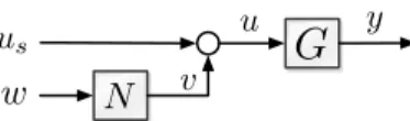
us
v u y N
G
w
Fig. 1. A typical interconnection ofGwith its nullspace generatorGo in a reconfiguration architecture
N(ρ,I)wassigns to the input signalw(t)the output response v(t)of the dynamical (LPV) system
N : x˙o=Ao(ρ)xo+Bo(ρ)w
v=Co(ρ)xo+Do(ρ)w , (7) where xo(0) = 0. Due to practical applicability we are interested in stable nullspace generator, therefore if N is not stable, it has to be stabilized. For this, we can use a similar factorization as (3). To proceed, we make assumption (iii):
there exists a stabilizing state feedback gain F(ρ) such that Ao(ρ) +Bo(ρ)F(ρ)is asymptotically stable. Then with
Mr(ρ,I) Nr(ρ,I)
=Fu
Ao(ρ) +Bo(ρ)F(ρ) Bo(ρ)
F(ρ) I
Co(ρ) +Do(ρ)F(ρ) Do(ρ)
,I
the equality N(ρ,I) = Nr(ρ,I)Mr(ρ,I)−1 holds so Nr(ρ,I)defines a stable generator system.
In the fault tolerant control framework the role ofN is to generate an input reconfiguration signal for G that does not influence its output. The general interconnection is depicted in Fig. 1.Gis assumed to be connected in a closed loop such that us is a stabilizing input generated by some (baseline) controller. Let us examine the system behavior in a practical situation, when the initial state ofGdiffers from zero and is not known either. Assume thatNis stable and starts from zero initial state. Since the systems are linear, Gis stabilized via us(t)andN is stable, the state transients generated due to the nonzero initial condition die out and the output ofGconverges to the response corresponding to us(t). Consequently, w(t) does not influencey(t).
Finally, assume that condition (i) does not hold, i.e.D(ρ) is not a full row rank matrix. We show that in this case the full row rank property can still be achieved by iteratively replacing the outputs causing rank deficiency by their time derivatives until a full row rank D0 matrix is obtained. This idea is the same as that is used in [20] for constructing the inverse of a linear system. The main steps of the procedure are summarized in the following algorithm. For simplicity, we present the procedure for LTI systems. The parameter-varying case can be similarly handled.
Algorithm 1. Assume for simplicity that[C D] has full row rank, i.e. the trivial output redundancy is excluded. LetC1= C,D1=D,y1=y andk= 1.
1) If Dk 6= 0 compute its SVD as Dk = [Uk,1 Uk,2]h
Σk 0 0 0
i hV∗
k,1
Vk,2∗
i, and perform a
linear transformation using the invertible matrix Uk∗: y˜k = Uk∗yk = hU∗
k,1Ckx+ ΣkVk,1∗ u Uk,2∗ Ckx
i = hC
k,1x+Dk,1u Ck,2x
i = hy˜
k,1
˜ yk,2
i
. Trivially, if Dk = 0,
theny˜k,2=yk and there is no y˜k,1.
2) Replacey˜k,2by its time derivative, i.e. let the new output equation be defined as follows:
yk+1=hC
k,1
Ck,2A
ix+hD
k,1
Ck,2B
iu=Ck+1x+Dk+1u.
3) Setk:=k+ 1. IfDk is of full row rank, then terminate and go to step 4. Otherwise, go to step 1.
4) Let the transformed system be defined as follows:
G0: x˙ =Ax+Bu
y=Ckx+Dku (8) If the algorithm terminates in finite steps, thenG0 can be con- structed. Since only derivations and invertible transformations are applied in each step,G0 has the same kernel as ofGand, by construction, Dk has full row rank. Consequently, (6) can be applied. The main concept of the algorithm can be extended to LPV systems, but in that case the transformed system will depend on the time derivatives of the scheduling parameters as well. As the generator computed from G0 inherits this dependence, the time derivatives of the parameters have to be known (measured or precisely computed) to evaluate the generator system.
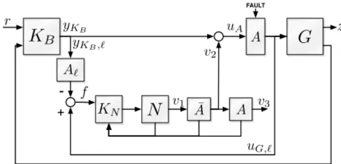
III. CONTROL INPUT RECONFIGURATION ARCHITECTURE FOR COMPENSATING ACTUATOR FAILURES
In this section an input reconfiguration method is proposed to compensate actuator failures. The concept extends the main idea of [8] to parameter varying systems that do not necessarily have static nullspace. The architecture presented in Figure 2 is similar to that proposed in [10], but the concept we follow is basically different.
Before proceeding, we introduce the following notational convention: If S denotes a dynamical system, then its `-th input and output will be denoted byuS,`andyS,`, respectively.
Let the nu input – ny output LPV plant be denoted by G.
Assume the actuators driving the inputs of Gare modeled by LTI systems collected in the nu input – nu output block A.
Let KB denote the baseline controller designed to guarantee the stability and control performance in fault-free case. For simplicity, consider now the case of one actuator fault affecting the`-th control input such thatuG,`=yA,`+f =A`(yKB,`)+
f, wheref is an external fault signal, A` is the`-th actuator dynamics. Suppose that uG,` (or equivalentlyf) is available for measurement or can be reconstructed by a suitable FDI filter, e.g. [21]. LetA¯be annuinput –nu output LTI shaping filter defined later and letN be the (stable) generator for the nullspace ofG·A·A. The procedure of input reconfiguration is¯ the following. If controllerKN is designed such thatv3,`(the
`-th component ofv3) tracks the fault signal f, then uA,`= yKB,`+v2,`, i.e.yA,`=A`(yKB,`) +A`(v2,`) =A`(yKB,`) + f =uG,`, i.e. the `-th output of the actuator block equals to the faulty input to the plant. Therefore it looks as if the faulty input had been generated by the baseline controller. The input reconfiguration is performed via v2, because it modifies the other control inputs such that they adapt to the faulty input.
Sincev2is generated from the nullspace, thus it does not have any effect on the plant’s behavior, i.e. the baseline control loop remains intact and the nominal control performance is preserved.
r z
FAULT
yKB,`
-
+ f
uG,ℓ v3 v1
v2 uA
¯ A
N
A KNA
G
A`
K
B yKBFig. 2. Input reconfiguration architecture
To complete the discussion, the role of the shaping filterA¯ remains to be clarified. This dynamical block can be chosen by the designer to shape the actuator dynamics in order to simplify the nullspace computation. For example, if A is invertible then one can chooseA¯=A−1and thus the actuators are eliminated from the reconfiguration procedure. IfAis not invertible, it may be possible to find an invertible A, whichˆ approximates A over the frequency range of its bandwidth.
ThenAˆ= ˆA−1 can be chosen. If the approximation does not work either,A¯ can still be chosen to ”advantageously shape”
the actuator dynamics. For example, [10] proposes to chooseA¯ such thatA·A¯=κ(s)I, whereκ(s)is a user-defined transfer function. This unification simplifies the generator system and can improve the conditioning of the numerical computations related to the construction ofN.
Finally, we add some comments and remarks to the archi- tecture above.
1) It is clear that the method works perfectly only if the exact model of the plant is known, since the kernel and the plant should perfectly match in order that the effect of the input reconfiguration on the control performance could be perfectly cancelled. If there is modelling uncertainty in the system, then the robustness of the reconfigured system has to be checked either by simulations or by using a classical analysis tool based on L2 gain computation and Integral Quadratic Constraints (IQC), see e.g. [22]. It is a possible option as well to improve the robustness properties of the reconfigured system by tuning the tracking controllerKN.
2) The design of the trajectory tracking controllerKN is not difficult in general as the states of every dynamical model in the reconfiguration block (i.e.N,A¯andA) are fully available.
Also, when modelling uncertainty is present the tracking controller can also be used to attenuate the performance degradation caused by the mismatch of the (nominal) nullspace and the (uncertain) plant. To handle this additional objective, this requirement has to be transformed to a performance target considered in the design ofKN.
3) The number and type of faults that can be compensated by the proposed method depend on the dimension and dynam- ical properties of the kernel space. If the dynamical properties are not appropriate (e.g. the kernel dynamics contain too fast or too slow dynamical components) the stabilizing state feedback gainF(ρ)or the tracking controllerKN can be used to shape this dynamics and set the required behaviour.
IV. RECONFIGURABLE FAULT TOLERANT CONTROL OF THE
B-1AIRCRAFT
The Rockwell B-1 Lancer is a supersonic bomber that was introduced in the 1970s. It has four turbofan engines and variable wing sweep. In order to analyze the aeroelastic issues occuring at subsonic speeds a high fidelity simulator was developed in [23].
A. The nonlinear flight simulator
To test the reconfigurable architecture in a realistic envi- ronment, the high-fidelity mathematical model is used. The simulator consists of the following main components: the nonlinear dynamics of the B-1 aircraft, the dynamics of the actuators and the stability augmentation system (SAS). In this case study the flexible components were neglected, only the rigid body dynamics were used. The simplified structure of the simulator is presented in Fig. 3.
The inputs to the nonlinear model are the left (L) and right (R) horizontal tails (uHR, uHL), wing upper-surface spoilers (uSP R, uSP L), splitted upper (RU) and lower (RL) rudders (uRU, uRL) and control vanes (uCV R, uCV L). All are measured in [deg]. Since the flexible part was neglected the control vanes appear as free inputs that can be used in actuator reallocation. This configuration corresponds to the subsonic, clean configuration case. The model has 10 states:
x = [φ, θ, ψ, p, q, r, u, v, w, h], where φ, θ, ψ are the roll-, pitch- and yaw angles in [rad], p, q, r are the corresponding angular rates in [rad/s],u, v, wdenote the body axis velocities in [ft/s] andhis the height in [ft]. The model is scheduled with height and the Mach numberM. The inner loop system has 4 outputs,y= [p, q, r, ay]T, whereay is the side acceleration measured in[g], which is often referred as side load factorny. The structure of the dynamics can be given as follows:
˙
x=F(ρ, x, u) y=
E4,5,6x h(ρ, x)
+
0
`(ρ, x)
u
where matrix E4,5,6 selects p, q, r from the state vector and h(ρ, x), `(ρ, x) are nonlinear functions defining ay. The scheduling variableρis a two dimensional vector comprising of the height and the Mach number, i.e. ρ = [h, M]. We assume that the flight envelope is defined such that ρ takes values only from polytopeΩ, defined by the following 4 ver- tices:[10000, 0.55],[10000, 0.7],[20000, 0.65],[20000, 0.8].
The actuators are modeled by first order linear systems with output saturation. The poles of the LTI models and the saturation limits are collected in Table I. The sensors dynamics are neglected from the present investigation due to their high bandwidth.
The SAS is responsible for the inner-loop rigid body control of the aircraft, providing pitch-, and roll-rate tracking and a yaw damper function using the measurements defined above and the reference stick commands from the pilot. In our reconfigurable control architecture the SAS is considered as the baseline controllerKB.
Actuator Poles Lower Lim. Upper Lim.
Horizontal tails −10,−57.14 −20deg 10deg Wing u/s spoilers −10,−20 0deg 45deg
Lower rudder −20,−80 −10deg 10deg
Upper rudder −10 −10deg 10deg
Control vanes −50 −20deg 20deg
TABLE I
PROPERTIES OF THE ACTUATORS
Actuator Dynamics
Nonlinear Aircraft
Model
SAS
uHR, uHL, uSP R, uSP L, uRU, uRL uCV R,
uCV L
h, M p, q, r, ay
Fig. 3. Basic configuration of the closed loop system
B. Construction of the LPV model
In order to construct the LPV model, the nonlinear dynamics are trimmed and linearized at different points of the flight envelope. By analyzing several configurations, we finally select 12 points equidistantly covering the Ω domain. After removing the unstable spiral mode from the model, least- squares interpolation is used to connect the 12 LTI systems into the following affine LPV model:
G(ρ,I) =Fu
A(ρ) B(ρ) C(ρ) D(ρ)
,I
, where (9)
A(ρ) =A0+A1h+A1M B(ρ) =B0+B1h+B1M C(ρ) =C0+C1h+C1M D(ρ) =D0+D1h+D1M The results are verified by computing the gap- and ν-gap metrics [24], [25] between (9) and the linearized models at the 14 grid points. Since none of the gap metrics exceed 0.025among the points, the LPV model is accepted as a good approximation of the original dynamics.
C. Actuator inversion and nullspace computation
Since the actuator dynamics are stable, they can be aug- mented with suitably fast left half plane zeros to make them biproper, and hence invertible. It is clear that the faster the zeros, the better the approximation is. On the other hand, arbitrarily fast zeros cannot be chosen because that would lead to high transients in the inverse dynamics. Therefore, as a compromise, the zeros are chosen to be four times faster than the poles in each actuator. Since the zeros are much faster than the bandwidth of the controller and the plant, the use of approximate inverses do not significantly influence the performance of the reconfigured control loop.
The next step is the computation of the nullspace ofG(ρ,I).
For this, the first three outputs p, q, r have to be derived because D(ρ)is not a full row rank matrix. After derivation, the rank condition is satisfied so no more derivations are necessary to determine the kernel. Since the output equations definingp,q andr do not depend onρ, the new outputsp,˙ q˙ andr˙ and consequently the kernel do not depend on ρ. The˙ kernel N(ρ,I) finally obtained is unstable, so it has to be stabilized. For this, following the formal coprime factorization
10−6 10−5 10−4 10−3 10−2 10−1 100 101 102
−240
−220
−200
−180
−160
−140
−120
−100
−80
−60
−40
Magnitude [dB]
Fig. 4. Bode plot of the systemsG(ρ,I)N(ρ,I)(blue) andG(ρ,I)N(ρ) (green) from the first input to the output q. Different lines correspond to different flight speed and height
method, a stabilizing state feedback F(ρ) is designed by solving the feasibility problem as follows:
A(ρ)Q+QA(ρ)T+
+B(ρ)Y +YTBT(ρ) + 2cQ≺0 hu2
limI Y YT Q
i0
(10)
whereQ=P−1,V(x) =xTP xis the Lyapunov function and constantsc, ulimare used to control the location of the poles (at fixedρvalues) and the norm of the feedback gain matrix, respectively [26]. The free variables in (10) areQandY from which the feedback gain is computed as F :=Y Q−1, which is now parameter-independent. (Parameter-dependent feedback gain can also be constructed by choosingQandY parameter- dependent.) To solve (10) the matrix inequalities are reduced to a finite set of LMI-s by evaluating them over a suitable dense grid overΩ[27].
We found in this particular example that the parameters c andulimcan be chosen such that the kernel dynamics become significantly slower than the closed loop formed by the plant and the baseline controller. This makes it possible to truncate the states and substitute the dynamical kernel by a static, parameter dependent feedthrough gain, i.e.N(ρ) :=Do(ρ). In order to analyze howN(ρ)”approximates” the true generator system the bode plots of G(ρ,I)N(ρ,I) and G(ρ,I)N(ρ) are computed for different values of ρ. The worst results are obtained from the first input of the kernel to the output q.
This input-output combination is shown in Fig. 4. It can be seen that G(ρ,I)N(ρ) is very close to zero in this case as well, soN(ρ)is a suitable approximation of the nullspace. It is important to emphasise that N(ρ) can not be determined without the dynamical kernel, because the augmented input matrix [B(ρ)T D(ρ)T]T has full column rank for all ρ∈Ω so it does not have a nullspace.
D. Fault signal tracking
The next component of the reconfigurable control architec- ture is the construction of theKN controller that is responsible for tracking the fault signal f = u` −A`(s)yKB,`, where u` is the output of the `-th (faulty) actuator and yKB,` is the `-th output of the baseline controller. Since the kernel
is static, this trajectory tracking problem is equivalent to finding for each time t a suitable uN(t) such that the `-th entry of N(ρ(t))uN(t) be equal to f(t). As we have strict and asymmetric constraints for the actuator outputs (Table I), this problem is solved by parameter-dependent quadratic programming (QP):
uminN(t)(r(t)−N(ρ(t))uN(t))TW(r(t)−N(ρ(t))uN(t))
w.r.t. N(ρ(t))uN(t)≥L−yKB
N(ρ(t))uN(t)≤U−yKB
(11) where the vector r of reference signals is defined as ri = 0 if i6=` andr` =f. Vectors L andU collect the lower and upper limits of the actuators and the diagonal matrixW is used to weight the tracking errors [8], [13]. By defining r in the way above we prescribe 0 reference for the non faulty inputs.
This expresses our intention to keep the healthy inputs close to the value determined by the baseline controller. By varying the entries of W the contribution of each control input to the reconfiguration signalyN can be tuned. (In the numerical simulations belowW = diag(w1, . . . , wnu)is used withw`= 1000andwi= 1 for i6=`, i.e. precise tracking is demanded for the fault signal but no preferences are prescribed for the use of other control inputs.
E. Simulation results
To demonstrate the applicability of the proposed recon- figurable control architecture the following fault scenario is presented: the pilot performs a pitch-rate doublet maneuver, by giving aqref command as shown in Fig. 6. The maneuver starts at t = 0sec. It is assumed that at t = 1sec the right horizontal tail is jammed at its actual position. By assuming an ideal fault detection and isolation algorithm, the reconfiguration starts also at t= 1sec.
Simulation results are shown for the healthy (green), faulty (blue), and for the reconfigured (red) cases in Figs. 5-7.
The roll rate response of the three cases are shown in Figure 5, where the ideal case of healthy behavior is constantly zero again, in case of a right horizontal tail fault roll rate excursions of 4 deg/s occur due to the asymmetrical deflections of the control surfaces. The proposed control allocation scheme is able to reduce it by at least a factor of four and the steady state error is zero, showing the clear advantage of the proposed method. The nonzero transient error is due to the nonlinear aircraft model. By testing the method on the LPV model only a negligibly small (less than 10−5) error can be experienced due to the numerical inaccuracy of the simulation and the use of approximate actuator inverse.
The main objective of pitch rate tracking in healthy, faulty and reconfigured cases are simulated in Figure 6. The healthy and reconfigured responses are very close to each other, while the uncompensated case have more than50%error and nonzero steady state error. This shows that, although stability is not lost, the performance of the uncompensated case in not acceptable.
The yaw rate response of the three cases are shown in Fig. 7, where it is clear that the healthy behavior does not
0 5 10 15
−3
−2
−1 0 1 2 3 4
p [deg / s]
Time (s)
Fig. 5. Simulation result of the angular ratepin three different cases: without fault (green dashed), with fault and reconfiguration (red solid), and with fault (blue dot-dashed)
0 5 10 15
−15
−10
−5 0 5 10 15 20
q [deg / s]
Time (s)
Fig. 6. Simulation result of the angular rateqin three different cases: without fault (green dashed), with fault and reconfiguration (red solid), and with fault (blue dot-dashed). The reference signalqref is plotted by solid blue.
leave the longitudinal plane, while the uncompensated case have small but non negligible yaw rate response. When the reconfiguration scheme is applied a similar fourfold transient response decrease can be seen, while the steady state error is improved by an order of magnitude. The nonzero error is again due to the nonlinear characteristics of the simulation, since in the LPV simulations the difference between healthy and compensated behaviors are not visible.
Fig. 8 - 10 show the inputs uHR, uHL, uSP R anduSP L
with and without reconfiguration. The contribution of the other inputs are small in all the simulation scenarios. It can be seen that the compensation of the faulty right horizontal tail required the active use of the left horizontal tail (uHL) and the two spoilers (uSP R, uSP L). The latter two are not used in normal operations.
F. Robustness analysis
As our reconfigurable control is based on perfect cancella- tion of the plant dynamics, the performance of the baseline controller can be perfectly preserved only if the exact plant model is known. Since in a real environment this condition is never met the performance of the reconfigured system always has to be checked for a set of models. Therefore, simulation are performed with different values of inertia and mass parameters of the aircraft. The nullspace based allocation and the tracking controller are held the same as in the nominal case. The actual
0 5 10 15
−0.2
−0.1 0 0.1 0.2 0.3 0.4 0.5 0.6 0.7 0.8
r [deg / s]
Time (s)
Fig. 7. Simulation result of the angular raterin three different cases: without fault (green dashed), with fault and reconfiguration (red solid), and with fault (blue dot-dashed)
0 5 10 15
−18
−16
−14
−12
−10
−8
−6
−4
−2 0
uHR [deg]
Time (s)
Fig. 8. Simulation result of the inputuHRin three different cases: without fault (green dashed), with fault and reconfiguration (red solid), and with fault (blue dot-dashed). The fault occurs at1sec
values of the parameters are selected randomly according to uniform distribution in a±20% interval around their nominal values of: Ixx = 950000, Ixz = −52700, Iyy = 6400000, Izz= 7100000,mass= 8944, where the inertia is measured in [sl.f t2] and the mass is given in [sl]. This way 500 different scenarios are generated and tested. The results are summarized in Fig. 11, where the angular rates are plotted for the 7 most representative parameter values. It can be seen that the results are very similar in all cases, leading to a conclusion that
0 5 10 15
−20
−15
−10
−5 0 5
uHL [deg]
Time (s)
Fig. 9. Simulation result of the inputuHLin three different cases: without fault (green dashed), with fault and reconfiguration (red solid), and with fault (blue dot-dashed). The fault occurs at1sec
0 5 10 15 0
1 2 3 4 5 6 7
uSPR, uSPL [deg]
Time (s)
Fig. 10. Simulation result of the two spoilersuSP RanduSP Lin the case of reconfiguration. These inputs are not used by the SAS. The fault occurs at 1sec
0 5 10 15
−10
−5 0 5 10 15 20
Time (s)
p, q, r [deg / s]
p q r
Fig. 11. Robustness analysis of the angular ratesp(blue),q(green),r(red)
the fault-tolerant controller is robust to the mass and inertia parameters.
V. CONCLUSION
A dynamic kernel based input reallocation framework has been proposed to accommodate actuator faults in LPV sys- tems. The method improves and extends the concept presented in [8]. Though the paper provides a complete design method, there are several points where the proposed approach can be further improved. First of all, the properties of the nullspace and the generator system have to be further analyzed in order to provide clear conditions for the stabilizability and well- definedness of the generator system and to find a systematic method for the right (or left) factorization. Second, the recon- figuration architecture provides large freedom for the designer:
the generator dynamics can be shaped by state feedback and the design method used to construct the tracking controller can be freely chosen. This freedom can be exploited to achieve further performance objectives, e.g. to improve the robustness properties of the closed-loop against modeling uncertainties.
These points assign research directions that should be focused on in the future.
ACKNOWLEDGMENT
The authors would like to thank Peter Seiler (University of Minnesota) and Arnar Hjartarson (formerly MUSYN Inc.) for
providing insight related to the B-1 simulator model, originally developed by David Schmidt.
REFERENCES
[1] P. Goupil and A. Marcos, “Industrial benchmarking and evaluation of addsafe fdd designs,” in Fault Detection, Supervision and Safety of Technical Processes (8th SAFEPROCESS), 2012.
[2] T. J. J. Lombaerts, Q. P. Chu, J. A. Mulder, and D. A. Joosten,
“Modular flight control reconfiguration design and simulation,”Control Engineering Practice, vol. 19, no. 6, pp. 540–554, 2011.
[3] I. Hwang, S. Kim, Y. Kim, and C. Seah, “A survey of fault detection, isolation, and reconfiguration methods,” Control Systems Technology, IEEE Transactions on, vol. 18, no. 3, pp. 636–653, 2010.
[4] P. Goupil, J. Boada-Bauxell, A. Marcos, E. Cortet, M. Kerr, and H. Costa, “Airbus efforts towards advanced real-time fault diagnosis and fault tolerant control,” in19th IFAC World Congress, Cape Town, South Africa, 2014, pp. 3471–3476.
[5] S. Ganguli, A. Marcos, and G. Balas, “Reconfigurable LPV control design for Boeing 747-100/200 longitudinal axis,” inAmerican Control Conference, vol. 5, 2002, pp. 3612–3617.
[6] H. Alwi, C. Edwards, and C. Tan,Fault Detection and Fault-Tolerant Control Using Sliding Modes. Springer-Verlag, 2011.
[7] T. A. Johansen and T. I. Fossen, “Control Allocation - A survey,”
Automatica, vol. 49, no. 5, pp. 1087–1103, 2013.
[8] L. Zaccarian, “Dynamic allocation for input redundant control systems,”
Automatica, vol. 45, pp. 1431–1438, 2009.
[9] D. Enns, “Control allocation approaches,” inAIAA GNC, 1998.
[10] A. Cristofaro and S. Galeani, “Output invisible control allocation with steady-state input optimization for weakly redundant plants,” inConfer- ence on Decision and Control (CDC), 2014, pp. 4246–4253.
[11] S. Galeani, A. Serrani, G. Varanoa, and L. Zaccarian, “On input allocation-based regulation for linear over-actuated systems,”Automat- ica, vol. 52, pp. 346–354, 2015.
[12] F. Wu and K. Dong, “Gain-scheduling control of LFT systems using parameter-dependent lyapunov functions,”Automatica, vol. 42, pp. 39–
50, 2006.
[13] B. Vanek, T. Peni, Z. Szab´o, and J. Bokor, “Fault tolerant LPV control of the GTM UAV with dynamic control allocation,” inAIAA GNC, 2014.
[14] A. Varga, “The nullspace method-a unifying paradigm to fault detec- tion,” in IEEE Conference on Decision and Control, 2009, pp. 6964–
6969.
[15] ——, “On computing nullspace bases - a fault detection perspective,”
in17th IFAC World Congress, 2008, pp. 6295–6300.
[16] J.-F. Magni. (2006) Linear Fractional Representation Toolbox for use with Matlab. [Online]. Available: http://w3.onera.fr/smac/?q=lfrt [17] R. D’Andrea and S. Khatri, “Kalman decomposition of linear fractional
transformation representations and minimality,” in American Control Conference (ACC), 1997, pp. 3557–3561.
[18] C. Beck and R. D’Andrea, “Noncommuting multidimensional realization theory: Minimality, reachability and observability,”IEEE Transactions on Automatic Control, vol. 49, no. 10, pp. 1815–1820, 2004.
[19] Z. Szab´o, T. P´eni, and J. Bokor, “Null-space computation for qLPV Systems,” in1st IFAC Workshop on Linear Parameter Varying Systems, 2015.
[20] L. M. Silverman, “Inversion of multivariable linear systems,” IEEE Transactions on Automatic Control, vol. AC-14, no. 3, pp. 270–276, 1969.
[21] H. Alwi, C. Edwards, and A. Marcos, “Actuator and sensor fault reconstruction using an LPV sliding mode observer,” in AIAA GNC, 2010.
[22] H. Pfifer and P. Seiler, “Robustness analysis of linear parameter varying systems using integral quadratic constraints,” International Journal of Robust and Nonlinear Control, vol. 25, pp. 2843–2864, 2015.
[23] D. Schmidt, “A nonlinear simulink simulation of a large flexible aircraft,”
MUSYN Inc. and NASA Dryden Flight Research Center, Tech. Rep., 2013.
[24] T. T. Georgiou, “On the computation of the gap metric,”Systems Control Letters, vol. 11, pp. 253–257, 1988.
[25] G. Vinnicombe, “Measuring robustness of feedback systems,” Ph.D.
dissertation, Department of Engineering, University of Cambridge, 1993.
[26] S. Boyd, L. E. Ghaoui, E. Feron, and V. Balakrishnan,Linear Matrix Inequalities in System and Control Theory, ser. Studies in Applied Mathematics. SIAM, 1994, vol. 15.
[27] F. Wu, “Control of linear parameter varying systems,” Ph.D. dissertation, University of California at Berkeley, 1995.