Tensor Product Model-Based Control for Space- craft with Fuel Slosh Dynamics
Hengheng Gong
1, Hang Sun
2, Binglei Wang
1, Yin Yu
3, Zhen Li
1,∗, Xiaozhong Liao
1, Xiangdong Liu
11School of Automation and Key Laboratory for Intelligent Control & Decision on Com- plex Systems, Beijing Institute of Technology, Beijing 100081, China.
2Shandong Institute of Aerospace Electronics Technology, Yantai, China.
3Science and Technology on Electronic Information Control Laboratory, Chengdu 610036, China.
Email: ghh9611@126.com; sunhang912@163.com; 1790261156@qq.com;
yuyin206@163.com; zhenli@bit.edu.cn; liaoxiaozhong@bit.edu.cn; xdliu@bit.edu.cn.
∗Corresponding author: zhenli@bit.edu.cn
Abstract: Large spacecrafts undertaking long-life mission greatly suffer from the nonlinear fuel slosh when altering the orbit or maneuvering, which leads to the downgrade on the per- formance and even stability of the body attitude control by unintentionally generating the huge disturbance thrust. In order to specifically address this solid-liquid coupling problem for a kind of spacecrafts when altering orbit, a nonlinear control method based on Ten- sor Product (TP) Model transformation is proposed to make a quick response control of the translational velocity vector and the attitude of the spacecraft. Based on the derived poly- topic system fromTP model transformation, the controller design can guarantee the robust against the uncertainties and disturbances for all system sets within the bounds. The pro- posed solution also offers an approximation tradeoff so that both the complexity of the TP model and the controller design can be dramatically minimized. The simulation results for spacecrafts with practical specification verify that the design method can make the spacecraft asymptotically stable and demonstrate the effectiveness of the proposed controller.
Keywords: Nonlinear control; TP model transformation; fuel slosh; high-order singular value decomposition.
1 Introduction
With the booming technology, the large spacecraft is undertaking more and more complicated applications with various kinds of higher requirements, which can be characterized by more on-orbit tasks and longer on-orbit time. In order to prolong
the lifetime of spacecraft and improve its stability, a large amount of liquid fuel must be carried. Hence, it will cause the fuel sloshing when the spacecraft alters the orbit or maneuvers with a partially full fuel tank. As a consequence, a disturbance torque on the spacecraft is generated by the fuel slosh. This solid-liquid coupling system presents the nonlinear and parameter time-varying characteristics. With the continuous consumption of fuel, the torque caused by slosh and the centroid offset could no longer be ignored for on-orbit tasks because the resultant huge jet thrust has an enormous impact on the stability of the attitude control, especially when the spacecraft alters its orbit. There are several typical failure experiences, which were caused by the fuel slosh [1].
To analyze and overcome this problem, the modeling is first of significance. The re- search on the fuel slosh model has two branches. The first one is based on the three- dimension models of various types [2,3,4,5], and the second is focused on planar models [6,7,8,9,10,11,12,13]. As for both of these models, the common purpose is to take place of the liquid by some masses. Thus, the dynamics can be described in an easier way. In terms of masses stated above, it can be further categorized into another two branches. For example, the slosh liquid is equivalent to a single pendu- lum in [2,3,5,6,8], and the other is using the mass-spring in [7,9,10,11,12,13].
The accuracy of both analytical approaches was experimentally evaluated to esti- mate model parameters [15]. Currently, the problem regarding attitude maneuvers was addressed using different methods, for example, dynamic inversion and input shaping control method [2], various feedback control based on PID, linear quadratic regulator (LQR) and linear quadratic Gaussian (LQG) method [6,7,8, 10,15].
Besides, a mechanical model was built based on Computational Fluid Dynamics (CFD) tools to estimate the propellant sloshing effect [11]. And a reduced-order observer was used in the full-state feedback in [12] for the estimation of the slosh states. The time-varying parameters were also considered in [13]. [16] presented a computational methodology based on Legendre’s polynomials to predict the slosh and acoustic motion in nearly incompressible fluids in both rigid and flexible struc- tures with free surface. []However, most of these method mentioned above just designed the parameters by rule of thumb so that it was difficult to provide the best options. Besides, the computational efficiency is still a prominent issue due to the real-time numerical solving for some methods. Although some improvements have been made for the complicated application, some methods still cannot afford computational burdens for the spacecraft application because the spacecraft is sig- nificantly constrained by the on-board computational resources. Therefore, it is still desirable to develop a high efficient method in computational resources.
The tensor-product (TP) model transformation is an alternative way to solve the optimized nonlinear control problem in view of the nonlinear model transforma- tion [17, 18,19, 20, 21], which is a numerical method and based on the high- order singular value decomposition (HOSVD) [23,24, 25]. Due to its universal approximation property, the TP model transformation is widely applied upon the original time varying nonlinear system. The resultant model is expressed in the convex combination form of the linear time invariant (LTI) systems. With the acquisition of the TP model, the subsequent linear controller design can be thus transformed to a convex optimization problem so that it can be numerically solved
based on a set of linear matrix inequalities (LMI). Since both the transformation and optimization can be carried out off-line in advance, the TP model transfor- mation method is therefore effective in alleviating the on-line computation [26].
On the other hand, the number of vertices and approximation error of TP model transformation can be effectively adjusted by varying the number of retained sin- gular values. Therefore, it can achieve a trade-off between approximation accu- racy and complexity [27], which has been already used in many nonlinear con- trols [28,26,29,30,31,32,33,34,35,36,37,38,39,40,41]. Hence, it is efficient and easy to be implemented.
In this paper, the altering orbit and maneuvering in planar are taken into considera- tion at the same time with the huge torque in zero gravity environment. A state feed- back controller based on Tensor-product (TP) model transformation is proposed for the control of the translational velocity vector and the attitude of the spacecraft. By means of the TP model transformation, the nonlinear slosh system model is trans- formed into thepolytopicsystem, which can be treated as a linear convex-bounded uncertain system. Therefore, the nonlinear slosh control problem is accordingly converted into linear matrix inequality (LMI) problem based on the quadratic Lya- punov stability theory. The advantage of our solution is that the converted LMI problem can be effectively solved by convex optimization methods. In addition, the proposed controller design method is robust against the uncertainties and dis- turbances since the controller keeps valid for all the system sets within the convex- bounded system obtained by the TP model transformation.
The remaining part is organized as follows. In Section II, the mass-spring model is described and simplified by the elimination of a mass from [15]. The detailed TP model transformation for the nonlinear slosh system are formulated in section III.
Section IV further gives the state feedback controller design and the solution via LMI. In Section V, the simulation example is presented to verify the effectiveness of the proposed control. Finally, Section VI concludes the paper.
2 The Solid-liquid Model of Fuel Slosh for Spacecrafts
m I0 0
h
b
d s
0
h
q
h
d vx
vz
M 2
k
k2
z O m1
Z X
x
F
Figure 1
The slosh mass-spring model for a spacecraft
The maneuvering control problem is under study for the spacecraft with single fuel tank in a zero gravity environment during its altering orbit. By considering the
movement of the spacecraft on a plane, the spacecraft can be physically described as a mass-spring model to formulate the dynamics, which is indicated in Fig.1.
In the axisymmetric model of Fig.1, two coordinates of Oxz, OX Z are established as the bodyframe and orbit coordinate system, respectively, andθdenotes the attitude angle between these two frames. vx,vz are the axial and transverse components of the velocity of the center of the fuel tank. The tank with fuel is modeled by the mass-spring, which has two components, i.e., the fixed and slosh parts. The fixed part has the mass of m0, whose moment of inertia is I0, and the sloshed part is with the mass of m1joined to the tank by two springs, whose elastic coefficients are k/2.
A restoring force −ks acts on the mass m1whenever the relative position to the z-axis s6=0. The locations h0>0,h>0 are referenced to the center of the tank.
A thrust F is produced by a gimballed thrust engine as shown in Fig.1, where δ denotes the gimbal deflection angle and is considered as one of the control inputs.
A pitching moment M is also available for the control purpose. There are some other constants in the problem statement such as the rigid spacecraft mass m, the moment of inertia I, the distance b between z-axis of the body coordinate and the spacecraft center of mass located along the longitudinal axis, the distance d from the gimbal pivot to the spacecraft center of mass, and the damping coefficient c of the spring.
Based on the formulation in [10], the equations of motion can be obtained as (m+mf)(˙vx+θ˙vz) +mb ˙θ2+m1(s ¨θ+2 ˙s ˙θ) =F cosδ (1) (m+mf)(˙vz−θ˙vx) +mb ¨θ+m1(¨s−s ˙θ) =F sinδ (2) I ¨ˆθ+m1[s(v˙x+θ˙vz)−h ¨s+2s ˙s ˙θ] +mb(v˙z−θ˙vx) =M+F(b+d)sinδ (3) m1(s¨+v˙z−θ˙vx−h ¨θ−s ˙θ2) +ks+c ˙s=0 (4) where
Iˆ=I+I0+mb2+m0h20+m1(h2+s2),mf =m0+m1.
Because the thruster F is quite large during altering orbit, it is reasonable to ignore the fuel slosh dynamics along x-axis such as the second order terms in (1). Be- sides, it is further assumed that the axial acceleration term ˙vx+θ˙vzis insignificantly changed since theθandδ vary within a small range compared with the impact from the thruster F along x-axis [10]. Consequently, the equation of (1) becomes,
˙
vx+θ˙vz= F m+mf
Let u1 u2
=D−1
"
F sinδ−m1(¨s−s ˙θ) M+F(b+d)sinδ−m1[s(m+mF
f)−h ¨s+2s ˙s ˙θ]
#
where D=
m+mf mb mb Iˆ
By the transformation from(δ,M)to two new control inputs(u1,u2),the system(1)- (4) can be rewritten as,
˙
vz=θ˙vx(t) +u1 (5)
θ¨=u2 (6)
¨
s=−ω2s−2ξωs˙+s ˙θ2−u1+hu2 (7)
whereω2=mk
1,2ξω=mc
1,ω andξ denote the undamped natural frequencies and damping ratios, respectively. Define the state variable xxx=
θ θ˙ s s˙ vz
T
and the whole system can be formulated by
xxx=fff(xxx,t) +bbb(xxx,t)uuu, (8) where
fff(xxx,t) =
θ 0
˙ s
−ω2s−2ξωs+˙ s ˙θ2 θ˙vx(t)
, and (9)
b bb(xxx,t) =
0 0
0 1
0 0
−1 h
1 0
With the model built above, the control objective is thus to design a nonlinear controller to accomplish a given planar maneuver. The equilibrium state xxxeq = θeq 0 0 0 veqz
and veqx . Without loss of generality, veqz =0,θeq=0, so the equilibrium point is xxx=xxxeq=000,vx=veqx .
3 TP Model Transformation for the Nonlinear Slosh System of Spacecrafts
This section transforms the nonlinear slosh system of spacecrafts into thepolytopic system by using TP model transformation, based on which the nonlinear slosh con- trol problem can be converted into linear matrix inequality (LMI) problem.
Consider the dynamical system modeled in state-space form
˙xxx(t) =AAA(p(t))xxx(t) +BBB(p(t))uuu(t) (10) where uuu(t)∈Rl and xxx(t)∈Rm are the input and state vectors, respectively. The system matrix is S(p(t)) =
AA
A(p(t)) BBB(p(t))
∈Rm×(m+l),where p(t)∈RN is time varying in the N-dimension bounded space Ω∈RN. Further, the parameter
p(t)may include some or all elements of xxx(t). Assume that there is a fixed polytope satisfying
S(p(t))∈ {S1,S2, . . . ,SI}={
∑
I i=1αiSi,αi≥0,
∑
I i=1αi=1} (11)
where the systems S1,S2, . . . ,SIare the vertex systems of S(p(t)). When the values αiare considered as the basis functions wi(p(t)),
S(p(t))≈
∑
I i=1wi(p(t))Si.
With the approximation of S(p(t))above, the dynamical system (10) takes the form
˙xxx(t) =
∑
I i=1wi(p(t))(AAAixxx(t) +BBBiuuu(t)) (12)
When the basis functions are decomposed for all dimensions to get a high order approximate decomposition, the TP model takes the form as
S(p(t))≈
I1
i
∑
1=1 I2i
∑
2=1· · ·
IN
iN
∑
=1∏
N n=1wn,in(pn(t))Si1,i2,...iN= S⊠Nn=1wwwn(pn(t))
(13)
where the values pn(t)are the elements of p(t)and normalized as below n∀n,pn(t):
In
in
∑
=1wn,in(pn(t)) =1,∀i,n,pn(t): wn,i(pn(t))≥0o .
Therefore, the system (10) can be transformed into
˙xxx(t)≈ S⊠Nn=1wwwn(pn(t))
xxx(t) u uu(t)
Accordingly, the remaining objective comes to how to solve the tensorS and the vector wwwn(pn(t)). Before the detailed demonstration of TP model transformation, various types of TP model will be discussed at first in the following subsection.
3.1 The Consideration of TP Model Types
The TP model for a given system is highly dependent on the construction of the weighting matrices regardless of the permutation of the vertices and the weighting functions. If satisfying the sum normalization (SN) and non-negative (NN) condi- tions, which ensure the convexity and are the necessities to the LMI-based methods, the TP model can be classified into the Normal (NO) type, close to the NO (CNO) type, the Inverted and Relaxed Normal (IRNO) type, and so on [22].
The feasibility of the LMIs solution is verified to be very sensitive to the structure of the TP model. It is obvious that the NO type is the most ideal candidate since it is as exact as the tight convex hull of the sampled system. However, it is impractical to obtain a strict NO result in the case of the limited number of the vertices. To ad- dress this issue, it is desirable to obtain a TP model in CNO type. However, the CNO variant of the TP model is again not unique and different CNO variants suffer from various degrees of conservativeness. Furthermore, in the case of INO-RNO type, it is guaranteed that the resultant vertex systems contributing in the convex combi- nation have equal distance to the system matrix S(p(t))in spaceΩΩΩ. Actually, the optimization for various types and their proper selection are still under discussion specific to different applications.
This paper focuses on the application of TP model transformation into the practi- cal aerospace control system, which features in the nonlinear characteristics. The optimization for one certain TP model types is not the main focus. Therefore, the INO-RNO type is applied in this paper to carry out the TP model transformation due to its feasibility.
3.2 The Implementation of TP Model Transformation
By using the INO-RNO type TP model representation [22,42], the polytopic ap- proximation can be calculated in the following steps. Assume the parameter p(t) varies within the bounded spaceΩΩΩ= [a1 b1]×[a2 b2]× · · · ×[aN bN]⊂RN. Step 1) Sampling the given functions over a hyper rectangular grid.
Define grid lines overΩon each vectors to get an N dimensional hyper rectangular grid. A simplest way is to set the lines evenly spaced, gn,mn =an+bMn−an
n−1(mn− 1),mn=1,2, . . . ,Mn.Then, calculate the system matrix S(p(t)) using the values sampled over the grid points SDm
1,m2,...,mn=S(pm1,m2,...,mn)∈Rm×(m+l).where pm1,m2,...,mn= (g1,m1,g2,m2, . . . ,gN,mN), and∀n : mn=1,2, . . . ,Mn. Next, using the tensorSD∈RM1×M2×···×MN×m×(m+l)to store the sampled value,(SD)m1,m2,...,mn= SDm
1,m2,...,mn.
Step 2) Computing the vertex systems matrices.
The HOSVD is executed to decomposeS as
SD=S⊠Nn=1Un. (14) After the decomposition, the tensorsS ∈RI1×I2×···×IN,Un∈RMn×Inand
In=rankn(SD)≤Mn, because of the ignorance of zero singular values. All the vertex systems Sm1,m2,...,mncan be obtained by using the processing according to the equation (13).
Step 3) Basis system normalization.
Normalize Unto Unfor satisfying the following conditions, which is described by
∑
(Un) =1Jn,un,jn,kn ≥0,
where 1Jn is Jndimensional column vector with all entries being 1.
Step 4) Basis function.
The values of the basis functions sampled over the grid points can be obtained by comparing the equations of (13) and (14)
wn,in(gn,mn) = (Un)mn,in (15)
So far, the TP model transformation is completed. wn,in(gn,mn)is used to approx- imate the wn,in(pn(t))over each subsection so that the bilinear approximation of S(p(t))is achieved.
4 Slosh Controller Design
Based on the TP model transformation for the nonlinear slosh system, this section presents the corresponding controller design.
Lemma 1. If a common matrix P>0 exists for all vertex systems with the condition AAATrP+PAAAr<0,r=1,2, . . . ,R. (16) Then, the equilibrium of TP model is globally and asymptotically stable.
Theorem 1. Consider the nonlinear system (8) and its polytopic approximation (12), if there exist matrix XXX>0 and matrices MMMrrr, r=1,2, . . . ,R solving the follow- ing linear matrix inequalities:
−XXX AAATr −AAArXXX+MMMTrBBBTr +BBBrMMMr>0,r=1,2, . . . ,R (17)
−XXX AAATr −AAArXXX−XXX AAATs −AAAsXXX+MMMTsBBBTr +BBBrMMMs+MMMTrBBBTs +BBBsMMMr≥0,1≤r<s≤R (18) then the continuous system is globally and asymptotically stable at the equilibrium by using the control input:
uuu(t) =−
∑
R r=1wr(p(t))FFFr
!
xxx(t), (19)
where FFFr=MMMrXXX−1. Proof:
By considering (19), (12) can be rewritten as
˙xxx(t) =
∑
R r=1∑
R s=1wr(p(t))ws(p(t))(AAAr−BBBrFFFs)xxx(t). (20)
With the assistance of defining a new matrix GGGr,s=AAAr−BBBrFFFs, in order to satisfy the condition of Lemma 1, there must have GGGTr,sP+PGGGr,s<0,r,s=1,2, . . . ,R.However,
this is a sufficient but not necessary condition. By the dedicated consideration of the control and calculation time, (20) can be divided into two components
˙xxx(t) =
∑
R r=1wr(p(t))wr(p(t))GGGr,rxxx(t) +
∑
R r=1∑
R s=r+1wr(p(t))ws(p(t)) (GGGr,s+GGGs,r)xxx(t).
The continuous system is globally and asymptotically stable in the large at the equi- librium if both parts satisfy Lemma 1. That is
GGGTr,rP+PGGGr,r<0, (21)
and
(GGGr,s+GGGs,r)TP+P(GGGr,s+GGGs,r)<0, (22) where r=1,2, . . . ,R and r<s≤R.
Hence, FFFr needs to be further determined to satisfy the condition of Lemma 1 re- garding a common positive-definite matrix P.
Define two new variables XXX=P−1>0 and MMMr =FFFrXXX , and then multiply the in- equalities of (21) and (22) on the left-hand side by XXX , we can get
−XXX AAATr −AAArXXX+MMMTrBBBTr +BBBrMMMr>0, (23)
−XXX AAATr −AAArXXX−XXX AAATs −AAAsXXX+MMMTsBBBTr +BBBrMMMs+MMMTrBBBTs +BBBsMMMr≥0. (24) By means of the transformation fromequations(21)-(22) toequations(23)-(24), the design is turned into an LMI problem,any other details could be found in [43]. The conditions are jointly convex in XXX and MMMrrr. Therefore, the positive-defined matrix XXX and MMMrrrneeds to be found in order to satisfy the conditions. Numerically, the com- putation of this problem can be efficiently solved by many available mathematical tools.
Remark. The main objective of this proposed control is to extend the practical appli- cation of TP model transformation into fuel slosh problem of spacecraft. Therefore, the simple model in [10] was applied. Although its polytopic model can be derived easily, the corresponding TP model transformation has more general application in practice. The design demonstrates the application of TP model transformation. It is also effective for the model more complex, e.g., multi-mass spring, which gives a higher accurate model information.
5 Verification with Numerical Simulation
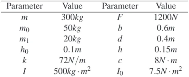
The physical parameters of the spacecraft with fuel slosh used in this part are given in Table1.
Table 1 Physical Parameters
Parameter Value Parameter Value
m 300kg F 1200N
m0 50kg b 0.6m
m1 20kg d 0.4m
h0 0.1m h 0.15m
k 72N/m c 8N·m
I 500kg·m2 I0 7.5N·m2
And fff(xxx,t)in (8) can be rewritten as fff(xxx,t) =AAA(xxx,t)xxx,where
AAA(xxx,vx(t)) =
0 1 0 0 0
0 s −θ˙ 0 0
0 0 0 1 0
0 s ˙θ −ω2 −2ξω 0
0 vx(t) 0 0 0
.
So the system (8) becomes
˙xxx(t) =AAA(xxx,vx(t))xxx(t) +BBBxxx(t). (25) Compared to the equation of(10), it is a special case with the constant matrix BBB.
A simplified system matrix is chosen so as to reduce the computational burden by S(p(t)) =AAA(xxx,vx(t)),wherep(t) =x2,x3,vx(t).
As the AAA(xxx,vx(t))is a state-dependent matrix, this form won’t be accompanied by an unique solution and there are many matrices matching the equation of (25). How- ever, the selection of AAA(xxx,t)will affect the controlled results and the computation complexity. Here, the value of AAA(xxx,t)depends on three states, i.e., ˙θ, s and vx(t).
As described in Section III, the first step is undertaken to sample the states above over a hyper rectangular grid. Here, give a rectangular grid in experience via many simulations.
si=−1+0.15i, i=1,2, . . . ,13.
vvvx,j=10+20 j, j=1,2, . . . ,20.
θθθ˙k=−2.2+0.2k, k=1,2, . . . ,22.
It turns out that the ranks of all the three dimensions are 2. Thus, by removing all the zero singular values in the step 2 of the TP model transformation, 8 vertex systems are remained,
AAA1=
0 1 0 0 0
0 −1 2.2 0 0
0 0 0 1 0
0 2.2 −1.8 −0.2 0
0 10 0 0 0
, AAA2=
0 1 0 0 0
0 −1 2.2 0 0
0 0 0 1 0
0 2.2 −1.8 −0.2 0
0 390 0 0 0
,
AAA3=
0 1 0 0 0
0 0.95 −2.2 0 0
0 0 0 1 0
0 2.09 −1.8 −0.2 0
0 390 0 0 0
, AAA4=
0 1 0 0 0
0 0.95 −2.2 0 0
0 0 0 1 0
0 2.09 −1.8 −0.2 0
0 10 0 0 0
,
AAA5=
0 1 0 0 0
0 −1 −2.2 0 0
0 0 0 1 0
0 −2.2 −1.8 −0.2 0
0 10 0 0 0
, AAA6=
0 1 0 0 0
0 −1 −2.2 0 0
0 0 0 1 0
0 −2.2 −1.8 −0.2 0
0 390 0 0 0
,
AAA7=
0 1 0 0 0
0 0.95 2.2 0 0
0 0 0 1 0
0 −2.09 −1.8 −0.2 0
0 390 0 0 0
, AAA8=
0 1 0 0 0
0 0.95 2.2 0 0
0 0 0 1 0
0 −2.09 −1.8 −0.2 0
0 10 0 0 0
,
BBB1−8=BBB.
The coefficient functions wrin equation (19) can be obtained by step 4 with 3 com- ponents (wr=wswvxwθ˙) as follows.And FFFr=MMMrXXX−1can be accordingly computed
s(m)
-1 -0.5 0 0.5 1
Weighting functions
0 0.2 0.4 0.6 0.8 1
vx(m/s)
0 100 200 300 400
Weighting functions
0 0.2 0.4 0.6 0.8 1
θ(rad)
-4 -2 0 2 4
Weighting functions
0 0.2 0.4 0.6 0.8 1
Figure 2 Three components of wr.
by equations (23)-(24).
FFF1=
0.0394 22.7069 −0.7180 0.3030 0.2137 0.1244 2.5719 4.4376 2.0346 −1.1604
, FFF2=
0.0324 −4.9377 −2.9289 −0.6519 1.4266 0.1129 0.7964 −3.9113 −0.4062 1.2638
, FFF3=
0.1002 406.0724 4.2298 14.7410 1.7203 0.2299 10.7266 15.7007 34.8356 2.1560
, FFF4=
0.0933 378.4343 2.0207 13.7864 2.9328 0.2184 8.9377 7.3511 32.3958 4.5811
, FFF5=
0.0389 23.5300 −0.7281 0.1577 0.1643 0.1234 4.4683 4.4233 1.7040 −1.2780
, FFF6=
0.0333 −4.0324 −2.8251 −0.4707 1.4099 0.1143 2.8825 −3.6701 0.0050 1.2209
, FFF7=
0.0997 406.9042 4.2245 14.5948 1.6669 0.2290 12.6282 15.6873 34.5060 2.0383
, FFF8=
0.0940 379.2346 2.1306 13.9589 2.9087 0.2196 11.0320 7.5916 32.7891 4.5341
.
By considering the influence of fuel burn into the parameters, the simulation time is chosen as 100 s and the altering thrust is stopped at 80 s. During this time slot, it is assumed that the fuel mass m0and m1are constant. Time responses shown in Fig.3 to Fig.5 correspond to the initial conditions ofθ0=0.55rad, ˙θ0=0, s0=0.1m,
˙
s0=0, vz0=20m/s. It can be seen from Fig.3and Fig.4, the transverse velocity
Time(s)
0 10 20 30 40 50 60 70 80 90 100
θ(rad)
-1 0 1
Time(s)
0 10 20 30 40 50 60 70 80 90 100
vz(m/s) -20
0 20
Time(s)
0 10 20 30 40 50 60 70 80 90 100
vx(m/s) 0 200 400
Figure 3
Time response ofθ,vzand vx.
vz, the attitude angleθ, the slosh state s converge to the relative equilibrium at zero
Time(s)
0 10 20 30 40 50 60 70 80 90 100
s(m)
-0.3 -0.2 -0.1 0 0.1 0.2 0.3
Figure 4
Time response of slosh state s.
Time(s)
0 10 20 30 40 50 60 70 80 90 100
δ(rad)
-1 -0.5 0 0.5 1
Time(s)
0 10 20 30 40 50 60 70 80 90 100
M(Nm)
-200 0 200 400
Figure 5
The inputs gimbal deflection angleδand pitching moment M.
and vxincreases as an uniformly accelerated motion. During the orbital transfer, the controller can stabilize the spacecraft within a time as short as 15 seconds.
Furthermore, a nonlinear direct feedback controller is developed for the comparison in performance such as the response time and overshot, the details of which were summarized and can be referred in [8,9,10]. The corresponding direct feedback controller is designed as follows.
u1=−2000h
5×10⁻⁵vz−0.002(s−h ˙θ)i ,
u2=− 1
10−0.002h2
80θ+1000 ˙θ+5×10⁻⁵vxvz+ 0.002(hsω2+h ˙sξ+s ˙s ˙θ−h ˙θ2s)
.
(26)
The objective of the slosh controller is to alleviate the impact from the fuel slosh dy-
Time(s)
0 10 20 30 40 50 60 70 80 90 100
vz(m/s) -20
0 20
Time(s)
0 10 20 30 40 50 60 70 80 90 100
θ(rad)
-1 0 1
Time(s)
0 10 20 30 40 50 60 70 80 90 100
s(m)
-0.5 0 0.5
FeedBack TP
Figure 6
The comparison between the direct feedback and TP controller, where the red dashed curve is corresponding to the direct feedback control and the blue solid one is for the TP control.
namics. Therefore, the response time (convergence) and overshot is of emphasis, the former of which determines how fast the controller eliminates the slosh dynamics.
Besides, a slighter overshot (a relative deviation along z-axis) reflects the gradual mitigation by the controller although the fast response is always accompanied with the smaller overshot. The performance is plotted and compared in Fig. 6, which show that the state s (a relative deviation along z-axis) gets convergent within 10 seconds and its corresponding overshot is also smaller than the direct feedback con- trol. Therefore, the proposed TP model-based control can achieve a faster response in convergence and slighter overshot so that the slosh dynamics can be effectively alleviated.
Conclusions
The paper proposes a numerical TP model transformation for space vehicles with fuel slosh. A state-dependent differential equation is firstly developed from the mass-spring model in zero gravity environment, which is transformed into thepoly- topicsystem and regarded as LMI problem. The advantage of our solution is that the converted LMI problem can be thus effectively solved by convex optimization methods. Based on the derivedconvex-bounded system, the controller design can always guarantee the robustness againstthe uncertainties and disturbances for all system sets within the bounds. Besides, this controller design is thus insuscep- tible to the time-varying parameters and coefficients seldom needs to be specially designed. Furthermore, the proposed TP model transformation offers an approxima- tion tradeoff so that both the complexity of the TP model and the controller design can be dramatically minimized.
Acknowledgement
This work was supported in part by National Natural Science Foundation of China under Grant Nos. 51407011 and 11572035, in part by Beijing Natural Science Foundation under Grant 3182034.
References
[1] Shageer, H. and G. Tao, “Modeling and adaptive control of spacecraft with fuel slosh: overview and case studies,” in Proc. AIAA Guidance, Navigation, and Control Conference, Hiton Head, South Carolina (2007).
[2] Baozeng, Y. and Z. Lemei, “Hybrid control of liquid-filled spacecraft ma- neuvers by dynamic inversion and input shaping,” AIAA J., vol. 52, no. 3, pp. 618–626 (2014).
[3] Baozeng, Y. and Z. Lemei, “Heteroclinic bifurcations in attitude maneuver of slosh-coupled spacecraft with flexible appendage,” J. of Astronautics, vol. 5, p. 007 (2011).
[4] Ayoubi, M. A., F. A. Goodarzi and A. Banerjee, “Attitude motion of a spin- ning spacecraft with fuel sloshing and nutation damping,” J. Astronaut. Sci. , vol. 58, no. 4, pp. 551–568 (2011).
[5] Kang, J.-Y. and S. Lee, “Attitude acquisition of a satellite with a partially filled liquid tank,” J. Guid. Control Dynam., vol. 31, no. 3, pp. 790–793 (2008).
[6] De Souza, A. G. and L. C. de Souza, “Satellite attitude control system design taking into account the fuel slosh and flexible dynamics,” Math. Probl. Eng., vol. 2014 (2014).
[7] Hervas, J. R., M. Reyhanoglu, and H. Tang, “Thrust-vector control of a three- axis stabilized spacecraft with fuel slosh dynamics,” in Proc. 13th Interna- tional Conference on Control, Automation and Systems (ICCAS), pp. 761–
766, IEEE (2013).
[8] Reyhanoglu, M., “Modelling and Control of Space Vehicles with Fuel Slosh Dynamics, Advances in Spacecraft Technologies,” Dr Jason Hall (Ed.), In- Tech (2011).
[9] Reyhanoglu, M. and J. R. Hervas, “Nonlinear dynamics and control of space vehicles with multiple fuel slosh modes,” Control Eng. Pract., vol. 20, no. 9, pp. 912–918 (2012).
[10] Reyhanoglu, M. and J. R. Hervas, “Nonlinear control of space vehicles with multi-mass fuel slosh dynamics,” in Proc. 5th International Conference on Recent Advances in Space Technologies (RAST), pp. 247–252, IEEE (2011).
[11] Dong, K., N. Qi, J. Guo and Y. Li, “An estimation approach for propellant sloshing effect on spacecraft gnc,” in Proc. 2nd International Symposium on Systems and Control in Aerospace and Astronautics, pp. 1–6, IEEE (2008).
[12] Hervas, J. R. and M. Reyhanoglu, “Observer-based nonlinear control of space vehicles with multi-mass fuel slosh dynamics,” in Proc. IEEE 23rd In- ternational Symposium onIndustrial Electronics (ISIE), pp. 178–182, IEEE (2014).
[13] Hervas, J. R. and M. Reyhanoglu, “Control of a spacecraft with time-varying propellant slosh parameters,” in Proc. 12th International Conference on Con- trol, Automation and Systems (ICCAS), pp. 1621–1626, IEEE (2012).
[14] Mitra, S., P. Upadhyay and K. Sinhamahapatra, “Slosh dynamics of invis- cid fluids in two-dimensional tanks of various geometry using finite element method,” Int. J. Numer. Meth. Fl., vol. 56, no. 9, pp. 1625–1651 (2008).
[15] Reyhanoglu, M., “Maneuvering control problems for a spacecraft with unac- tuated fuel slosh dynamics,” in Proc. IEEE Conference on Control Applica- tions (CCA), vol. 1, pp. 695–699, IEEE (2003).
[16] Krishna Kishor, D., S. Gopalakrishnan and R. Ganguli, “Three-dimensional sloshing: A consistent finite element approach,” Int. J. Numer. Meth. Fl., vol. 66, no. 3, pp. 345–376 (2011).
[17] P. Baranyi: “TP-Model Transformation-Based-Control Design Frame- works, Springer International Publishing Switzerland, 2016, p. 258. (eBook 978-3-319-19605-3, 978-3-319-19604-6, doi: 10.1007/978-3-319-19605-3, http://www.springer.com/gp/book/9783319196046)
[18] A. Szollosi, P. Baranyi Influence of the Tensor Product Model Representation Of QLPV Models on The Feasibility of Linear Matrix Inequality, Asian J.
Control, 2016, pp 1328–1342
[19] A. Szollosi, and P. Baranyi, Improved control performance of the 3-DoF aeroelastic wing section: a TP model based 2D parametric control perfor- mance optimization, Asian J. Control, vol. 19, no. 2, pp 450-466, 2017 [20] A Szollosi, P. Baranyi “Influence of the Tensor Product Model Representa-
tion of qLPV Models on the Feasibility of Linear Matrix Inequality Based Stability Analysis , Asian J. Control, 2017, in print
[21] X. Liu, L. Li, L. Zhen, T. Fernando, and H. H. C. Iu, “Stochastic stability condition for the extended kalman filter with intermittent observations,” IEEE Trans. Circuits Syst. II, Exp. Briefs, vol. 64, no. 3, pp. 334–338, March 2017.
[22] Baranyi, P., Yam Y. and V´arlaki P., “Tp model transformation as a way to lmi- based controller design,” Taylor & Francis, Boca Raton FL, pp. 248, 2013 (ISBN 978-1-43-981816-9).
[23] De Lathauwer, L., B. De Moor and J. Vandewalle, “A multilinear singular value decomposition,” SIAM J. Matrix Anal. A., vol. 21, no. 4, pp. 1253–
1278 (2000).
[24] Pan, J. and L. Lu, “Tp model transformation via sequentially truncated higher-order singular value decomposition,” Asian J. Control, vol. 17, no. 2, pp. 467–475 (2015).
[25] Baranyi, P., “The Generalized TP Model Transformation for TS Fuzzy Model Manipulation and Generalized Stability Verification” IEEE Trans. Fuzzy Syst., vol. 22, no. 4, pp. 934–948 (2014).
[26] Baranyi, P., “Tensor product model-based control of two-dimensional aeroe- lastic system,” J. Guid. Control Dynam., vol. 29, no. 2, pp. 391–400 (2006).
[27] Baranyi, P., P. Korondi, R. J. Patton and H. Hashimoto, “Trade-off between approximation accuracy and complexity for ts fuzzy models,” Asian J. Con- trol, vol. 6, no. 1, pp. 21–33 (2004).
[28] Baranyi, P., “Output feedback control of two-dimensional aeroelastic sys- tem,” J. Guid. Control Dynam., vol. 29, no. 3, pp. 762–767 (2006).
[29] Baranyi, P. and Takarics, B., “Aeroelastic Wing Section Control via Relaxed Tensor Product Model Transformation Framework” J. Guid. Control Dynam., vol. 37, no. 5, pp. 1671–1678 (2014).
[30] Takarics and B., Baranyi, P., “Tensor-Product-Model-Based Control of a Three Degrees-of-Freedom Aeroelastic Model,” J. Guid. Control Dynam., vol. 36, no. 5, pp. 1527–1533 (2013).
[31] Petres, Z., P. Baranyi, P. Korondi and H. Hashimoto, “Trajectory tracking by tp model transformation: case study of a benchmark problem,” IEEE Trans.
Ind. Electron.,, vol. 54, no. 3, pp. 1654–1663 (2007).
[32] Baranyi, P., “Tp model transformation as a manipulation tool for qlpv analy- sis and design,” Asian J. Control, vol. 17, no. 2, pp. 497–507 (2015).
[33] Campos, V. C. D. S., L. A. B. Tˆorres and R. M. Palhares, “Revisiting the tp model transformation: Interpolation and rule reduction,” Asian J. Control, vol. 17, no. 2, pp. 392–401 (2015).
[34] P. Baranyi, Z. Petres, P. Korondi, Y. Yam and H. Hashimoto, “Complexity relaxation of the Tensor Product Model Transformation for Higher Dimen- sional Problems,” Asian J. Control, vol. 9, no. 2, pp. 195–200 (2007).
[35] D. Tikk, P. Baranyi and R. J. Patton, “Approximation Properties of TP Model Forms and its Consequences to TPDC Design Framework,” Asian J. Control, vol. 9, no. 3, pp. 221–231 (2007).
[36] Sz. Nagy, Z. Petres, P. Baranyi and H. Hashimoto, “Computational relaxed TP model transformation: restricting the computation to subspaces of the dynamic model,” Asian J. Control, vol. 11, no. 5, pp. 461–475 (2009).
[37] P. Baranyi, P. Korondi and H. Hashimoto, “Global Asymptotic Stabilisation of the Prototypical Aeroelastic Wing Section via TP Model Transfromation,”
Asian J. Control, vol. 7, no. 2, pp. 99–111 (2005).
[38] X. Liu, L. Li, Z. Li, X. Chen, T. Fernando, H. H. C. Iu and G. He. “Event- trigger particle filter for smart grids with limited communication bandwidth infrastructure,” IEEE Trans. on Smart Grid, vol. PP, no. 99, pp. 1-1 (2017).
[39] S. Li, L. Li, Z. Li, X. Chen, T. Fernando, Herbert H. C. Iu, G. He, Q. Wang and X. Liu, “Event-trigger Heterogeneous Nonlinear Filter for Wide-area Measurement Systems in Power Grid,” IEEE Trans. Smart Grid, vol. PP, no.
99, pp. 1–1 (2018).
[40] B. Liu , Z. Li, X. Chen, Y. Huang and X. Liu, “Recognition and Vulnerability Analysis of Key Nodes in Power Grid Based on Complex Network Central- ity,” IEEE Trans. Circuits Syst. II, Exp. Briefs, vol. 65, no. 3, pp. 346–350 (2018).
[41] Y. Yu, Z. Li, X. Liu, K. Hirota, X. Chen, T. Fernando, and H. H. Iu, “A nested tensor product model transformation,” IEEE Trans. Fuzzy Syst., vol. PP, no.
99, pp. 1–1 (2018).
[42] X. Liu, Y. Yu, Z. Li, and H. H. Iu, “Polytopic H∞filter design and relaxation for nonlinear systems via tensor product technique,” Signal Process., vol.
127, pp. 191–205 (2016).
[43] Tanaka K, Wang H O. Fuzzy Control Systems Design and Analysis: A Linear Matrix Inequality Approach [M]. John Wiley & Sons, Inc. 2002.