Ostorcsapás-hatás elemzése egy HMMS típusú ellátási láncban
Dobos Imre
92. sz. Műhelytanulmány
HU ISSN 1786-3031
2008. június
Budapesti Corvinus Egyetem Vállalatgazdaságtan Intézet Fővám tér 8.
H-1093 Budapest Hungary
Műhelytanulmányok Vállalatgazdaságtan Intézet
1093 Budapest, Fővám tér 8., 1828 Budapest, Pf. 489 (+36 1) 482-5424, fax: 482-5567, www.uni-corvinus.hu/vallgazd
The analysis of bullwhip effect in a HMMS-type supply chain
Imre Dobos
Corvinus University of Budapest, Institute of Business Economics, H-1093 Budapest, Fővám tér 8., Hungary, imre.dobos@uni-corvinus.hu
Abstract. The aim of the paper is to investigate the well-known bullwhip effect of supply chains. Control theoretic analysis of bullwhip effect is extensively analyzed in the literature with Laplace transform. This paper tries to examine the effect for an extended Holt- Modigliani-Muth-Simon model. A two-stage supply chain (supplier-manufacturer) is studied with quadratic costs functional. It is assumed that both firms minimize the relevant costs. The order of the manufacturer is delayed with a known constant. Two cases are examined:
supplier and manufacturer minimize the relevant costs decentralized, and a centralized decision rule. The question is answered, how to decrease the bullwhip effect.
Keywords: Optimal control, Supply chain, Bullwhip effect
Absztrakt. A dolgozat célja a jólismert ostorcsapás-hatás elemzése ellátási láncokban. Az ostorcsapás-hatás irányításelméleti vizsgálata széleskörően ismert az irodalomban a Laplace- transzformáltak segítségével. Ez a dolgozat megkísérli újra vizsgálni a hatást egy kiterjesztett Holt-Modigliani-Muth-Simon modellben. Egy kétfázisú ellátási láncot (beszállító-termelő) vizsgálunk kvadratikus költségek mellett. Feltételezzük, hogy mindkét vállalat minimalizálja a költségeit. A termelő megrendelése egy ismert konstansnak megfelelően késik. Két esetet vizsgálunk: a beszállító és a termelő centralizáltan, vagy decentralizáltan minimalizálja a költségeket. Arra a kérdésre keressük a választ, hogyan csökkenthető az ostorcsapás-hatás.
Kulcsszavak: Optimális irányítás, Ellátási lánc, Ostorcsapás-hatás
1. Introduction
Bullwhip effect refers to the connections in supply chains. This effect explains the fluctuations of sales (demand), manufacturing, and supply. It was first observed by Forrester (1961) when studying industrial dynamics. Lee et al. (1997) have newly discovered this phenomenon. They have mentioned four basic causes of bullwhip effect:
- Forrester effect, or lead-times and demand signal processing, - Burbidge effect, or order batching,
- Houlihan effect, or rationing and gaming, and - promotion effect, or price fluctuations.
These new names after known scientists have been given by Disney et al. (2003).
Modeling of bullwhip effect was first made by Metters (1997). He has developed a stochastic model to discuss the fluctuations. Other stochastic modeling of the effect was fulfilled by e.g.
Cachon (1999), Kelle et al. (1999), Chen et al. (2000), Machuca et al. (2004), and Pujawan (2004) in an EOQ-environment. Chen et al. (2000) have explicitly proven that variation ratio of demand and manufacturing is strictly greater, than one, i.e. the fluctuations are increasing along the supply chains. These investigations examine the Forrester and Burbidge effects. A new direction in analysis of bullwhip effect is to apply fuzzy logic instead of stochastic modeling. (Carlsson et al. (2000), (2001))
Deterministic and control-theoretic investigations of bullwhip effect are made by Dejonckheere et al. (2003), Disney et al. (2003) and Geary et al. (2006).
In this paper we will examine the bullwhip effect in a HMMS-type supply chain. Holt, Modigliani, Muth, and Simon (1960) have developed a quadratic production planning model which was tested in a paint factory. In the last years the HMMS model is newly analysed extensively in the literature. (Dobos (2003), Singhal et al. (2007), and Atici et al. (2008)) The aim of the paper is to investigate a HMMS-type (Holt el al. (1960)) two-stage supply chain, and to analyse whether the bullwhip effect appears in this model. To show the bullwhip effect, we develop two models: a decentralized and a centralized HMMS-type supply chain models. The model is a continuous time control theoretic model with quadratic cost functional.
The paper organizes as follows. The decentralized model is presented in Section 2. In this section we pose the used model and we solve it. The next section discusses the centralized supply chain model with its solution. Sections 2 and 3 contain numerical examples to demonstrate the results. Lat we summarize the results of the paper.
2. The basic model: decentralized system
We examine a simple supply chain. The supply chain contains two firms, a supplier and a manufacturer. We assume that the firms are independent, i.e. they make decision to minimize their own costs. The firms have two stores: a store for raw materials and a store for end products. We will assume that the input stores are empty, i.e. the firms can order suitable
quantity, and they get the ordered quantity. The production processes have a known, constant lead time. The material flow of the model is depicted in Fig. 1.
The following parameters are used in the models:
T length of the planning horizon,
S(t) the rate of demand, continuous differentiable, t∈
[ ]
0,T ,τm lead time of manufacturing process, τs lead time of supply process,
) (t
Im inventory goal size of manufactured product, t∈
[ ]
0,T , )(t
Is inventory goal size of supplied product, t∈
[
−τm,T −τm]
, )(t
Pm manufacturing goal level, t∈
[ ]
0,T , )(t
Ps supply goal level, t∈
[
−τm,T −τm]
,hm inventory holding coefficient in manufactured product store, hs inventory holding coefficient in supplied product store, cm production cost coefficient for manufacturing,
cs production cost coefficient for supply.
Decision variables:
) (t
Im inventory level of manufactured product, non-negative, t∈
[ ]
0,T , )(t
Is inventory level of supplied product, non-negative, t∈
[
−τm,T −τm]
, )~( t
Is new inventory level of supplied product, non-negative, t∈
[ ]
0,T , )(t
Pm rate of manufacturing, non-negative, t∈
[ ]
0,T , )(t
Ps rate of supply, non-negative, t∈
[
−τm,T −τm]
, )~( t
Ps new rate of supply, non-negative, t∈
[ ]
0,T .The decentralized model examines a situation when the supplier and the manufacturer decide independently. It means that the manufacturer determines its optimal production-inventory strategy then it orders the necessary quantity of products to meet the known demand. The supplier accepts the order, and it minimizes the relevant costs. The cost function of supplier and manufacturer consists of two parts: quadratic production and inventory costs.
Figure 1. Material flow in the models
Im(t)
Supplier Manufacturer
Production Production
Pm(t-τm) Pm(t)
Pm(t-τm) Ps(t)
Ps(t-τs) Ps(t-τs)
Is(t)
S(t)
Let us now model the manufacturer in this HMMS-environment. (See Holt-Modigliani-Muth- Simon (1960)) The first decision is made by the manufacturer, and then the supplier determines the optimal production policy. The manufacturer will minimize the quadratic costs, as follows:
T t I
I t S t P t
I&m( )= m( )− ( ), m(0)= m0, 0≤ ≤ , (1)
[ ] [
( ) ( )]
min) 2 ( ) 2 (
0
2
2 →
− + −
∫
h I t I t c P t P t dtT
m m
m m
m
m . (2)
Let us assume that the optimal production-inventory policy of manufacturer is
(
Io(t),Pmo(t))
m
in model (1)-(2). The manufacturer orders Pmo(t+τm) to meet the manufacturing needs. The supplier must solve the next problem (3)-(4) to satisfy the order of manufacturer:
m m
s m s m o m s
s t P t P t I I t T
I& ( )= ( )− ( +τ ), (−τ )= 0, −τ ≤ ≤ −τ , (3)
[ ] [
( ) ( )]
min) 2 ( ) 2 (
2
2 →
− + −
−
∫
−
dt t P t c P t I t h I
m
m
T
s s
s s
s s τ τ
. (4)
Let us now transform the stock-flow equation of supplier in time:
, 0
), ( ) 0
~( ), ( )
~( )
~(
T t I
I t P t P t
I&s = s − m s = s −τm ≤ ≤ (5)
and goal functional
[
I t I t]
c[
P t P t]
dtT h
m s s
s m
s s
∫
s − − + − − 0
2
2 ~( ) ( )
) 2 (
)
~(
2 τ τ , (6)
where the new decision variables are ) ( )
~( ), (
)
~(
m s s
m s
s t I t P t P t
I = −τ = −τ .
We will solve the problem (5)-(6) instead model (3)-(4). The problem has the same planning horizon [0,T], as model (1)-(2).
Lemma 1. Let us assume that production-inventory strategy
(
I (t),Pmo(t))
o
m is an optimal solution for model (1)-(2). Then the optimal solution must satisfy the following differential equation:
⋅
−
−
+
⋅
=
) ( )
(
) ( )
( ) ( 0
1 0 )
( ) (
t c I
t h P
t S t
P t I c
t h P
t I
m m m o m
m o m
m o m
m o
m & &
&
&
,
with initial and ending value
) ( ) ( , ) 0
( I 0 P T P T
Imo = m mo = m .
We will not prove the lemma the proof can be found in paper Dobos (2003). If production strategy )Pmo(t is known, than problem (5)-(6) can be solved.
Lemma 2. Let us assume that production-inventory strategy
(
I~o(t),P~so(t))
s is an optimal
solution for model (5)-(6). Then the optimal solution must satisfy the following differential equation:
⋅
−
−
+
⋅
=
) ( )
(
) ( )
~ (( )
~ 0 1 0 )
~ (( )
~
t c I t h P
t P t
P t I c
h t
P t I
s s s s
o m o
s o s
s o s
s o
s & &
&
&
,
with initial and ending value ) ( )
~ ( , ) 0
~ (
0 P T P T
I
Iso = s so = s .
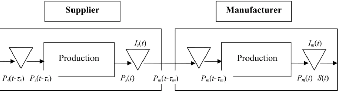
Example 1. The data of the example are in the appendix of this paper. For the data the optimal solution of model (1)-(2) is shown in Fig. 2. and Fig 3. Smoothness of a trajectory can be defined, as the difference between maximal and minimal values of this function. The manufacturing and supply rates seem to be smoother, than the demand rate for this example.
Smoothness of demand, manufacturing, and supply rates are equal to 2.000, 1.823, and 1.767.
But the manufacturing inventory level is much smoother than that of supplier. Smoothness of manufacturing inventory level is 0.404, and that of supply inventory level is 0.525.
0 200 400 600 800 1000
0.5 1 1.5 2 2.5 3
Pmmt
Psmt
S tT n .
t
Figure 2. Optimal manufacturing and supply rates for decentralized models
0 200 400 600 800 1000 0.2
0 0.2 0.4 0.6
Immt
Ismt
0
t
Figure 3. Optimal manufacturing and supply inventory levels for decentralized models
3. A new model: the centralized system
Now we solve models (1)-(2), and (5)-(6) simultaneously, i.e. the manufacturer and supplier make decision together. The form of this model is:
T t t
S t P t
I&m( )= m( )− ( ), 0≤ ≤ , (7)
, 0
), ( )
~( )
~(
T t t
P t P t
I&s = s − m ≤ ≤ (8)
=
0 0
) 0
~((0)
s m s
m
I I I
I . (9)
The goal functional is
[ ] [ ] [ ] [~() ( )]
min.
) 2 ( )
~( ) 2
( ) 2 ( ) ( ) 2 (
0
2 2 2
2 →
− + − + − − + − −
∫
h I t I t c P t P t h I t I t c P t P t dtT
m s s s m s s s m
m m m
m
m τ τ (10)
The Hamiltonian of model (7)-(10) is
[ ] [ ] [ ] [ ]
[
( ) ( )]
( )[
~( ) ( )]
) (
) ( )
~( ) 2
( )
~( ) 2
( ) 2 (
) ( ) 2 (
)) ( ), ( ),
~( ),
~( ), ( ), ( (
2 2 2
2
t P t P t t
S t P t
t P t c P t
I t h I t P t c P t I t h I
t t t P t I t P t I H
m s
s m
m
m s s
s m
s s
s m
m m m
m m
s m s s m m
− +
− +
+
−
−
−
−
−
−
−
−
−
−
=
ψ ψ
τ τ
ψ ψ
Lemma 3. Necessary and sufficient conditions of optimality of production-inventory strategy are
(
I (t),P (t),~Io(t),P~so(t))
s o m o
m :
1)
[
( ) ( )]
( )) (
)) ( ), ( ),
~ ( ),
~ ( ), ( ), (
( h I t I t t
t I
t t t P t I t P t I H
m m
o m m m
s m o s o s o m o
m ψ ψ ψ
&
−
=
−
−
∂ =
∂ ,
[
~ ( ) ( )]
( ))
~( ~ ( ), ( ), ( )) ),
~ ( ), ( ), (
( h I t I t t
t I
t t t P t I t P t I H
s m
s o
s s s
s m o s o s o m o
m ψ ψ τ ψ
&
−
=
−
−
−
∂ =
∂ ,
2)
[
( ) ( )]
( ) ( ) 0,) (
)) ( ), ( ),
~ ( ),
~ ( ), ( ), (
( =− − + − =
∂
∂ c P t P t t t
t P
t t t P t I t P t I H
s m
m o
m m m
s m o s o s o m o
m ψ ψ ψ ψ
[
~ ( ) ( )]
( ) 0,)
~( ~ ( ), ( ), ( )) ),
~ ( ), ( ), (
( =− − − + =
∂
∂ c P t P t t
t P
t t t P t I t P t I H
s m s o
s s s
s m o s o s o m o
m ψ ψ τ ψ
3) (T)− (T)=c
[
Po(T)−Pm(T)]
=0,m m s
m ψ
ψ ( )=
[
~o( )− s( − m)]
=0.s s
s T c P T P T τ
ψ
The optimal centralized production strategies for manufacturer and supplier are ),
( ) 1 ( ) 1 ( )
( t P t
t c t c
P s m
m m
m o
m = ψ − ψ +
and
).
( ) 1 ( )
~ (
m s s
s o
s t P t
t c
P = ψ + −τ
These two equations are the optimal linear decision rules. Differentiating adjoint variables )
m(t
ψ and ψs(t), and then substituting into conditions, the necessary and sufficient conditions become a system of linear differential equations:
−
−
−
− +
−
−
+
⋅
−
−
=
) ( )
(
) ( )
( )
(
0 ) (
)
~ (() )
~ (()
0 0 0
0 0
1 1 0
0
0 1 0 0
)
~ (( ) )
~ (()
m s s s m s
m s m
s m
m m m
o s
o m o s
o m
s s
m s m
m
o s
o m o s
o m
t c I t h
P
t c I t h c I t h P
t S
t P
t P
t I
t I
c h
c h c
h
t P
t P
t I
t I
τ τ
τ
&
&
&
&
&
&
(11)
with initial and ending values
=
0 0
) 0
~((0)
s m s
m
I I I
I ,
and
) . (
) ( )
~ (( )
= −
m s
m o
s o m
T P
T P T
P T P
τ
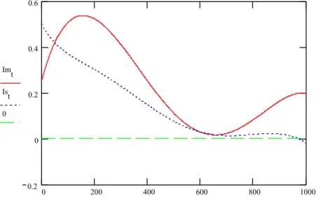
Example 2. For the known data the optimal solution of model (7)-(10) is shown in Fig. 4. and Fig 5. The manufacturing and supply rates seem to be smoother, than the demand rate for this example. Smoothness of demand, manufacturing, and supply rates are equal to 2.000, 1.86, and 1.732. In this example the manufacturing inventory level is not smoother than that of supply. Smoothness of manufacturing inventory level is 0.521, and that of supply inventory level is 0.5.
0 200 400 600 800 1000
0.5 1 1.5 2 2.5 3
Pmt
Pst
S t T n .
t
Figure 4. Optimal manufacturing and supply rates for centralized model
0 200 400 600 800 1000
0.2 0 0.2 0.4 0.6
Imt
Ist
0
t
Figure 5. Optimal manufacturing and supply inventory levels for centralized model
4. Conclusion
In this paper we have solved two two-stage supply chain models: a decentralized and a centralized model. Because of the quadratic costs, the necessary conditions of optimality are sufficient, as well. In decentralized model we have shown an example, where the supply, manufacturing, and demand fluctuations are decreasing along the supply chain. The same
proposition can be said in centralized model. In centralized model the costs are lower than that of in decentralized model. In centralized model the inventory levels are lower comparing manufacturing to supply.
Summarizing, in HMMS-environment fluctuations of flow variables are decreasing along the supply chain, but inventory levels fluctuate increasingly.
References
1. Atici, F. M., Uysal, F. (2008): A production-inventory model of HMMS on time scales, Applied Mathematics Letters 21, 236-243
2. Cachon, G. P. (1999): Managing supply chain demand variability with scheduled ordering policies, Management Science 45, 843-856
3. Carlsson, Ch, Fullér, R. (2001): Reducing the bullwhip effect by means of intelligent, soft computing methods, In: Proceedings of the 34th Hawaii International Conference on System Sciences – 2001, 1-10
4. Carlsson, Ch., Fullér, R. (2000): A fuzzy approach to bullwhip effect, In: Cybernetics and Systems 2000, Proceedings of the Fifteenth European Meeting on Cybernetics and Systems Research, Vienna, April 25-28, 2000, Austrian Society for Cybernetic Studies, 228-233
5. Chen, F., Drezner, Z., Ryan, J. K., Simchi-Levi, D. (2000): Quantifying the bullwhip effect in a simple supply chain: The impact of forecasting, leadtimes, and information, Management Science 46, 436-443
6. Dejonckheere, J., Disney, S. M., Lambrecht, M. R., Towill, D. R. (2003): Measuring and avoiding the bullwhip effect: A control theoretic approach, European Journal of Operational Research 147, 567-590
7. Disney, S. M., Towill, D. R. (2003): On the bullwhip and inventory variance produced by an ordering policy, Omega: The International Journal of Management Science 31, 157-167
8. Dobos, I. (2003): Optimal production-inventory strategies for a HMMS-type reverse logistics system, Int. J. of Production Economics 81-82, 351-360
9. Forrester, J. (1961): Industrial dynamics, MIT Press, Cambridge, MA
10. Geary, S., Disney, S. M., Towill, D. R. (2006): On bullwhip in supply chains – historical review, present practice and expected future impact, Int. J. of Production Economics 101, 2-18
11. Holt, C.C., Modigliani, F., Muth, J.F., Simon, H.A. (1960): Planning Production, Inventories, and Work Forces, Prentice-Hall, Englewood Cliffs, N.J.
12. Kelle, P., Milne, A. (1999): The effect of (s,S) ordering policy on the supply chain, Int. J. of Production Economics 59, 113-1212
13. Lee, H. L., Padmanabhan, V., Whang, S. (1997): The bullwhip effect in supply chains, Sloan Management Review, Spring, 93-102
14. Machuca, J. A. D., Barajas, R.P. (2004): The impact of electronic data interchange on reducing bullwhip effect and supply chain inventory costs, Transportation Research Part E 40, 209-228
15. Metters, R. (1997): Quantifying the bullwhip effect in supply chains, Journal of Operations Management 15, 89-100
16. Pujawan, I N. (2004): The effect of lot sizing rules on order variability, European Journal of Operational Research 159, 617-635
17. Singhal, J., Singhal, K. (2007): Holt, Modigliani, Muth, and Simon’s work and its role in the renaissance and evolution of operations management, Journal of Operations Management 25, 300-309
Appendix
Description Data
Length of planning horizon: T 5
Demand rate: S(t) sin(t)+2
Delay of the supply: τ 0.5
Manufacturing rate goal level: P tm( ) 1.0
Supply rate goal level: Ps(t) 0.85
Inventory size goal level in manufacturing store: Im(t) 0.5 Inventory size goal level in supply store: Is(t) 0.3
Manufacturing cost coefficient: cm 1.0
Supply cost coefficient: cs 0.5
Inventory holding coefficient in manufacturing store: hm 2 Inventory holding coefficient in supply store: hs 1 Table 1. Parameter specification for the example