Cooperation in an HMMS-type supply chain: A management application of cooperative game theory = Kooperáció egy HMMS-típusú ellátási láncban: A kooperatív játékelmélet egy menedzsment alkalmazása

Mőhelytanulmányok Vállalatgazdaságtan Intézet

1093 Budapest, Fıvám tér 8.

(+36 1) 482-5566, Fax: 482-5567

www.uni-corvinus.hu/vallgazd

Cooperation in an HMMS-type supply chain: A management application of

cooperative game theory

Imre Dobos Miklós Pintér

135. sz. M ő helytanulmány HU ISSN 1786-3031

2010. november

Budapesti Corvinus Egyetem Vállalatgazdaságtan Intézet

Fıvám tér 8.

H-1093 Budapest Hungary

Cooperation in an HMMS-type supply chain: A management application of cooperative game theory

Imre Dobos¹ Miklós Pintér²

1 Corvinus University of Budapest, Institute of Business Economics, H-1093 Budapest, Fıvám tér 8., Hungary, imre.dobos@uni-corvinus.hu.

2 Corvinus University of Budapest, Department of Mathematics, H-1093 Budapest, Fıvám tér 13-15., Hungary, miklos.pinter@uni-corvinus.hu.

Absztrakt

A cikkben a kooperatív játékelmélet fogalmait alkalmazzuk egy Holt-Mogigliani-Muth- Simon-típusú ellátási lánc esetében. Az ostorcsapás-hatás elemeit egy beszállító-termelı ellátási láncban ragadjuk meg egy kvadratikus készletezési és termelési költség mellett.

Feltételezzük, hogy mindkét vállalat minimalizálja a releváns költségeit. Két mőködési rendszert hasonlítunk össze: egy hierarchikus döntéshozatali rendszert, amikor elıször a termelı, majd a beszállító optimalizálja helyzetét, majd egy centralizált (kooperatív) modellt, amikor a vállalatok az együttes költségüket minimalizálják. A kérdés úgy merül fel, hogy a csökkentett ostorcsapás-hatás esetén hogyan osszák meg a részvevık ebben a transzferálható hasznosságú kooperatív játékban a költség megtakarítást, exogén módon adott tárgyalási pozíció mellett.

Kulcsszavak: Optimális irányítás, Ellátási lánc, Ostorcsapás-hatás, Kooperatív játékelmélet

Abstract

We apply cooperative game theory concepts to analyze a Holt-Modigliani-Muth-Simon (HMMS) supply chain. The bullwhip effect in a two-stage supply chain (supplier- manufacturer) in the framework of the HMMS-model with quadratic cost functions is considered. It is assumed that both firms minimize their relevant costs, and two cases are examined: the supplier and the manufacturer minimize their relevant costs in a decentralized and in a centralized (cooperative) way. The question of how to share the savings of the decreased bullwhip effect in the centralized (cooperative) model is answered by the weighted Shapley value, by a transferable utility cooperative game theory tool, where the weights are for the exogenously given “bargaining powers” of the participants of the supply chain.

Keywords: Optimal control, Supply chain, Bullwhip effect, Cooperative game theory, Weighted Shapley value

1 Introduction

In the supply chain literature so far mostly non-cooperative game theory concepts were applied, see e.g. Kogan and Tapiero (2007) and Sethi at al. (2005), for an exception see.

Dobos and Pintér (2010). In this paper we analyze supply chains by cooperative game theory tools. Our main question is that how the manufacturer and the supplier should share the savings they achieve by harmonizing their production plans. We apply the following cooperative game theory concepts: the core (Gillies (1959)) and the weighted Shapley value (Shapley (1953)) to answer the above question. The core concept expresses that the considered allocation of the savings is stable, while the weights in the weighted Shapley value are for the exogenously given “bargaining powers” of the participants of the supply chain, that is, those describe how the participants share the savings as a function of their “bargaining powers”.

In order to demonstrate the efficiency of cooperating in a supply chain we consider the so called bullwhip effect. The bullwhip effect explains the fluctuations of sales (demand), manufacturing and supply. The bullwhip effect was first observed by Forrester (1961), later Lee et al. (1997) rediscovered this phenomenon. They mentioned four basic causes of the bullwhip effect: lead-times and demand signal processing, order batching, rationing and gaming; and promotion effect, or price fluctuations. These effects were investigated e.g. by Disney et al. (2003).

There are three basic models to investigate the decision processes of a firm: the Wagner-Whitin, Arrow-Karlin and the Holt-Modigliani-Muth-Simon (HMMS) model. These models have a stock-flow identity and a cost function. The difference between them lies in the cost functions. The well-known lot sizing model of Wagner and Whitin (1958) assumes a concave cost function. The basic model of Arrow and Karlin (1958) applies a linear holding and a convex production cost function. The model of Holt, Modigliani, Muth and Simon (1960) assumes a quadratic function for both the inventory holding and the production cost.

The main goal of this paper is to demonstrate that the weighted Shapley value (Shapley (1953)), a cooperative game theory tool, can be applied to supply chain analysis. We consider an HMMS-type two-stage supply chain and analyse the bullwhip effect appearing in this model. To show that because of the bullwhip effect the cooperation of the manufacturer and the supplier induces savings, we develop two models: a decentralized and a centralized HMMS-type supply chain model.

The decentralized model assumes that first the manufacturer solves her production planning problem (the market demand is given exogenously) and her ordering process is based on the optimal production plan. Then the supplier minimizes her costs on the basis of the ordering of the manufacturer. In the centralized model it is assumed that the participants of the supply chain cooperate, that is, they minimize the sum of their costs.

In the next step we compare the production-inventory strategies and the costs of the manufacturer and supplier in the two models to show that the bullwhip effect can be reduced by cooperation (centralized model). This cooperation can be defined as a kind of information sharing between the parties of the supply chain.

Finally, we discuss the question of how the manufacturer and the supplier should share the savings their cooperation induces. We assume that the “bargaining powers” of the participants are given by weights summing up to one, and share the savings according to these weighs. We demonstrate that, in this model this concept coincides with the weighted Shapley value (Shapley (1953)) and it is stable, that is, it is in the core (Gillies (1959)).

The main differences between this paper and Dobos and Pintér (2010) are as follows:

(1) Dobos and Pintér (2010) consider the Arrow-Karlin model (Arrow and Karlin (1958)), while in this paper we analyze the Holt-Modigliani-Muth-Simon model, so the two papers

consider different management science situations. Moreover, (2) Dobos and Pintér (2010) assume that the manufacturer and the supplier have the same “bargaining powers”, that is, none of them can be considered as stronger than the other. In business, however, typically one of the participants is stronger than the other, that is, they do not have same “bargaining powers”. In other words, it is desirable to take care about the participants’ “bargaining powers” when we discuss the allocation of the savings achieved by the cooperation. In this paper, we apply the weighted Shapley value, in which the weights reflect the participants’

different “bargaining powers”.

The paper is organized as follows. The decentralized model is discussed in Section 2.

Section 3 analyzes the centralized (cooperative) supply chain model. In Section 4 we introduce some concepts of cooperative game theory and define supply chain (cooperative) games given by the models discussed in Sections 2 and 3. Moreover, we apply the above mentioned solution concepts of transferable utility cooperative games to answer the question of how the manufacturer and the supplier should share the savings, the result of their cooperation. An exact number example is given in Section 5. The last section briefly concludes.

2 The decentralized system

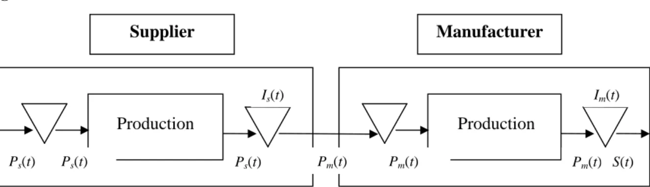
We consider a simple supply chain consisting of two firms: a supplier and a manufacturer. We assume that the firms are independent, that is, each makes her decision to minimize her own costs. The firms have two stores: a store for raw materials and a store for end products.

Moreover, we assume that the input stores are empty, that is, the firms can order suitable quantity and that they can get the ordered quantity. The production processes have a known, constant lead time. The material flow of the model is depicted in Figure 1.

Figure 1. Material flow in the models

The following parameters are used in the models:

T length of the planning horizon,

S(t) the rate of demand, continuous differentiable, ^t∈

[ ]

^{0,T ,}

) (t

I_m inventory goal size of manufactured product, ^t∈

[ ]

^{0,T ,}

) (t

I_s inventory goal size of supplied product, ^t∈

[ ]

^{0,T ,}

) (t

P_m manufacturing goal level, ^t∈

[ ]

^{0,T ,}

) (t

P_s supply goal level, ^t∈

[ ]

^{0,T ,}

h_m inventory holding cost coefficient in manufactured product store, hs inventory holding cost coefficient in supplied product store, cm production cost coefficient for manufacturing,

I_m(t)

Supplier Manufacturer

Production Production

P_m(t) Pm(t)

P_m(t) Ps(t)

P_s(t) P_s(t)

I_s(t)

S(t)

In the HMMS-model it is assumed that the management of the (manufacturer and supplier) firms have fixed a production-inventory pattern, that is, the production plans P_m(t) and P_s(t), and planned inventory levels I_m(t) and I_s(t) are known before the planning horizon. The objective of the managers of the firms is to minimize the deviations from the fixed objective level. The deviations are defined, as quadratic functionals with known parameters. This phenomenon was empirically tested by Holt, Modigliani, Muth, and Simon (1960).

The decision variables:

) (t

I_m the inventory level of the manufactured product, it is non-negative, ^t∈

[ ]

^{0,T ,}

) (t

I_s the inventory level of the supplied product, it is non-negative, ^t∈

[ ]

^{0,T ,}

) (t

P_m the rate of manufacturing, it is non-negative, ^t∈

[ ]

^{0,T ,}

) (t

P_s the rate of supply, it is non-negative, ^t∈

[ ]

^{0,T .}

The decentralized model describes the situation where the supplier and the manufacturer optimize independently, we mean the manufacturer determines its optimal production- inventory strategy first (the market demand is given exogenously), then she orders the necessary quantity of products to meet the known demand. Then the supplier accepts the order and minimizes her own costs.

Next, we model the manufacturer in this HMMS-environment. The manufacturer solves the following problem:

[ ] [

^{( ) ( )}

]

^min

) 2 ( ) 2 (

0

2

2 →







 − + −

=

∫

^{h I t I t c P t P t dt}

J

T

m m

m m

m m

m (1)

s.t.

T t I

I t S t P t

I&_m( )= _m( )− ( ), _m(0)= _m0, 0≤ ≤ (2)

Assume that the optimal production-inventory policy of the manufacturer is

(

^{Imd(⋅),Pmd(⋅)}

)

in model (1)-(2) and the manufacturer orders P_m^d(⋅). Then the supplier solves the following problem:

[ ] [

^{( ) ( )}

]

^min

) 2 ( ) 2 (

0

2

2 →







 − + −

=

∫

^{h I t I t c P t P t dt}

J

T

s s

s s

s s

s (3)

s.t.

T t I

I t P t P t

I&_s( )= _s( )− _m^d( ), _s(0)= _s0, 0≤ ≤ (4)

Notice that problem (3)-(4) has the same planning horizon [0,T] as that of model (1)- (2).

To solve problem (1)-(2) we apply the Pontryagin’s Maximum Principle (see e.g.

Feichtinger and Hartl, (1986), Seierstad and Sydsaeter, (1987)). The Hamiltonian function of this problem is as follows:

( ) [ ] [

^{( ) ( )}

]

^{( )}

(

^{( ) ( )}

)

^.

) 2 ( ) 2 ( ),

( ), ( ),

( ² c P t P t ² t P t D t

t I t h I t

t t P t I

H_{m m m m} ^m _{m m} ^m _{m m} + _m ⋅ _m −







 − + −

−

= ψ

ψ

This problem is an optimal control problem with pure state variable constraints. To obtain the necessary and sufficient conditions of optimality we need the Lagrangian function:

(

^{I (t),P (t), (t), (t),t}

)

^H

(

^{I (t),P (t), (t),t}

) ( ) ( )

^{t I t .}

L_{m m m} ψ_m λ_m = _{m m m} ψ_m +λ_m ⋅ _m

Lemma 1

(

^{Imd(⋅),Pmd(⋅)}

)

is the optimal solution of problem (1)-(2) if and only if there exists continuous function ψ_m(⋅) such that for all 0≤ ^t≤ ^T ψ_m⁽t⁾≠^{0 and}

(a)

( ) ( )

( ) ( )

^{t h}

[

^{I t I t}

] ( )

^t

t I

t t t t P t I

t L _{m m m}^d _{m m}

m

m m d m d m m

m ψ λ

∂ ψ λ

ψ =−∂ ( ), ( ), ( ), ( ), ⇒ = ( )− ( ) −

&

& ,

(b)

( )

{ } ( )

( )

{ } [ ^{( )}

^{( )}

]

^,

) 2 ( ) ( ),

( ), ( ), ( max

), ( ), ( ), ( ),

( ), ( ), ( max

2 0

) ( 0 ) (

t P t c P t P t t

t t P t I H

t t t P t I H t t t P t I H

d m d

m m d

m m m

m d m t m

P

m d m d m m m

m d m t m

P

m m

−

−

⋅

=

⇒

=

≥

≥

ψ ψ

ψ ψ

(c)

( ) ( )

^{t ⋅I t =0,} m

( )

^{t ≥0}

d m

m λ

λ ,

(d)

( ) ( )

^{T ⋅I T =0,} m

( )

^{T ≥0.}

d m

m ψ

ψ

We do not prove the above lemma, its proof can be found in the above mentioned literature.

The optimal solution can be easy constructed, if the optimal production rate and the optimal inventory level is positive in along the planning horizon.

Lemma 2 Assume that production-inventory strategy

(

^{Imd(⋅),Pmd(⋅)}

)

is an optimal solution for model (1)-(2). Then the optimal solution must satisfy the following differential equation:

















⋅

−

−

+











⋅











=













) ( )

(

) ( )

( ) ( 0

1 0 )

( ) (

t c I

t h P

t S t

P t I c

h t

P t I

m m m d m

m d m

m d m

m d

m & &

&

&

,

with initial and terminal condition

) ( ) ( , ) 0

( I ₀ P T P T

I_m^d = _{m m}^d = _m .

We do not prove this lemma, the proof can be found in Dobos (2003). If production strategy )

(

P_m^d ⋅ is known, then problem (3)-(4) can be solved.

After optimal production strategy P_m^d(⋅) is given we can solve problem (3)-(4). The Hamiltonian function of problem (3)-(4) is as follows

( ) [ ] [

^{( ) ( )}

]

^{( )}

(

^{( ) ()}

)

^.

) 2 ( ) 2 ( ),

( ), ( ),

( ² c P t P t ² t P t P t

t I t h I t

t t P t I

H_{s s s s} ^s _{s s} ^s _{s s} + _s ⋅ _s − _m^d







 − + −

−

= ψ

ψ

This problem is also an optimal control problem with pure state variable constraints.

To get the necessary and sufficient conditions of optimality, we need again the Lagrangian function:

(

^{I (t),P(t), (t), (t),t}

)

^H

(

^{I (t),P(t), (t),t}

) ( ) ( )

^{t I t.}

L_{s s s} ψ_s λ_s = _{s s s} ψ_s +λ_s ⋅ _s

The proof of the following lemma can be found again in the mentioned literature.

Lemma 3

(

^(⋅), s^d(⋅)

)

d

s P

I is optimal solution of problem (3)-(4), if and only if there exists continuous function ψ_s(⋅) such that for all 0≤ ^t≤ ^T ψ_s⁽t⁾≠^{0 and}

(a)

( ) ( )

( ) ( )

^{t h}

[

^{I t I t}

] ( )

^t

t I

t t t t P t I

t L _{s s s}^d _{s s}

s

s s d s d s s

s ψ λ

∂

λ ψ

ψ =−∂ ( ), ( ), ( ), ( ), ⇒ = ( )− ( ) −

&

& ,

(b)

( )

{ } ( )

( )

{ } [

^{( ) ( )}

]

^,

) 2 ( ) ( ),

( ), ( ), ( max

), ( ), ( ), ( ),

( ), ( ), ( max

0 ) ( 0 ) (

t P t c P t P t t

t t P t I H

t t t P t I H t t t P t I H

s d

s d s

s s s

s d s t s

P

s d s d s s s

s d s t s

P

s s

−

−

⋅

=

⇒

=

≥

≥

ψ ψ

ψ ψ

(c)

( ) ( )

^{t ⋅I t =0,} s

( )

^{t ≥0}

d s

s λ

λ ^,

(d)

( ) ( )

^{T ⋅I T =0,} s

( )

^{T ≥0.}

d s

s ψ

ψ

For the case of positive inventory level and production rate the optimal strategy is presented in the next lemma.

Lemma 4 Let us assume that production-inventory strategy

(

^(⋅), s^d(⋅)

)

d

s P

I is an optimal solution for model (3)-(4). Then the optimal solution must satisfy the following differential equation:

















⋅

− + −











⋅











=













) ( )

(

) ( )

( ) ( 0

1 0 ) (

) (

t c I t h P

t P t

P t I c

h t

P t I

s s s s

d m d

s d s

s d s

s d

s & &

&

&

,

with initial and terminal condition

) ( ) ( , ) 0

~ (

0 P T P T

I

I_s^d = _{s s}^d = _s ^.

Later we use the following notations: let J and _m^d J be the optimal values of cost _s^d functions (1) and (3) respectively, that is, let

[

^{I t I t}

]

^c

[

^{P t P t}

]

^dt

J h

T

m d

m m m

d m d m

m ⁼

∫

_^{ − + −} _^

0

2

2 ( ) ( )

) 2 ( ) 2 (

and

[

^{I t I t}

]

^c

[

^{P t P t}

]

^dt

J h

T

s d

s s s

d s d s

s ⁼

∫

_^{ − + −} _^

0

2

2 ( ) ( )

) 2 ( )

2 ( ^.

3 The centralized system

In this section we solve the centralized model, that is, the model, where the manufacturer and supplier coordinate their decisions. The model is as follows

[ ] [ ] [ ] [

^{() ()}

]

^min

) 2 ( ) 2 ( ) ( ) 2 ( ) ( ) 2 (

0

2 2

2

2 →







 − + − + − + −

=

∫

^{h I t I t c P t P t h I t I t c P t P t dt}

J

T

s s s s

s s m

m m m

m m

ms (5)

s.t.

T t t

S t P t

I&_m( )= _m( )− ( ), 0≤ ≤ (6)

, 0

), ( ) ( )

(t P t P t t T

I&_s = _s − _m ≤ ≤ (7)







=









0 0

) 0 (

) 0 (

s m s

m

I I I

I (8)

The Hamiltonian function of model (5)-(8) is

[ ] [ ] [ ] [ ]

[

^{( ) ( )}

]

^{( )}

[

^{( ) ( )}

]

^.

) (

) ( ) 2 ( ) ( ) 2 ( ) ( ) 2 ( ) ( ) 2 (

)) ( ), ( ), ( ), ( ), ( ), ( (

2 2

2 2

t P t P t t

S t P t

t P t c P t I t h I t P t c P t I t h I

t t t P t I t P t I H

m s

s m

m

s s

s s

s s m

m m m

m m

s m s s m m

−

⋅ +

−

⋅ +







 − + − + − + −

−

=

ψ ψ

ψ ψ

The Lagrangian function is

( )

(

^{( ), ( ), ( ), ( ), ( ), ( ),}

) ( ) ( ) ( ) ( )

^.

), ( ), ( ), ( ), ( ), ( ), ( ), ( ), (

t I t t

I t t

t t t P t I t P t I H

t t t t t t P t I t P t I L

s s m m s

m s s m m

s m s m s s m m

⋅ +

⋅ +

= ψ ψ λ λ

λ λ ψ ψ

The following lemma formalizes the well-known optimality conditions. Its proof can be found in the literature mentioned in the previous section.

Lemma 5

(

^{(⋅), (⋅), (⋅),} s^c(⋅)

)

c s c m c

m P I P

I is optimal solution of problem (5)-(8), if and only if the following points hold

1)

( )

[

^{( ) ( )}

]

^{( )( ) (),}

), ( ), ( ), ( ), ( ), ( ), ( ), ( ), (

t t

t I t I h

t I

t t t t t t P t I t P t I L

m m

m c

m m

m

s m s m c s c s c m c m

ψ λ

λ λ ψ ψ

&

−

= +

−

−

=

∂

∂

( )

[ ( )

^{( )}

]

^{( ) ( ) ( ),}

), ( ), ( ), ( ), ( ), ( ), ( ), ( ), (

t t

t I t I h

t I

t t t t t t P t I t P t I L

s s

s c s s

s

s m s m c s c s c m c m

ψ λ

λ λ ψ ψ

&

−

= +

−

−

=

∂

∂

2)

( )

{ }

( ) [

^{( ) ( )}

]

^,

) 2 ( ) ( ) (

), ( ), ( ), ( ), ( ), ( ), ( max

2 0

) (

t P t c P t P t t

t t t t P t I t P t I H

m c

m c m

m s

m

s m c s c s m c t m

P_m

−

−

⋅

−

=

≥

ψ ψ

ψ ψ

( )

{ }

[

^{( ) ( )}

]

^,

) 2 ( ) (

), ( ), ( ), ( ), ( ), ( ), ( max

2 0

) (

t P t c P t P t

t t t t P t I t P t I H

s c

s c s

s s

s m s c s c m c t m

P_s

−

−

⋅

=

≥

ψ

ψ ψ

3)

( ) ( )

^{t ⋅I t =0,} m

( )

^{t ≥0}

c m

m λ

λ ^,

( ) ( )

^{t ⋅I t =0,} s

( )

^{t ≥0}

c s

s λ

λ ^,

4)

( ( )

^{T −}

( )

^T

) ( )

^{⋅I T =0,} m

( )

^{T ≥0.}

c m s

m ψ ψ

ψ

( ) ( )

^{T ⋅I T =0,} s

( )

^{T ≥0.}

c s

s ψ

ψ

The optimal centralized production strategies for the manufacturer and the supplier respectively are

( ) ( )

( ) ( ) ( ) ( )









>

− +

− +

≤

− +

=

, 0 ) ( ),

(

, 0 ) ( ,

0 )

(

t c P

t if t

t c P

t t

t c P

t if t

t P

m m

s m

m m

s m

m m

s m

c

m ψ ψ ψ ψ

ψ ψ

and

( )

( ) ( )









>

+ +

≤ +

=

, 0 ) ( ),

(

, 0 ) ( ,

0 )

(

t c P

if t t c P

t

t c P

if t t

P

s c s s

c s

s c s c

s ψ ψ

ψ

These two equations are the optimal linear decision rules. (See Holt-Modigliani-Muth-Simon (1960).) Differentiating adjoint variables ψ_m(⋅) ^and ψs⁽⋅⁾, and then substituting into the conditions, the necessary and sufficient conditions become a system of linear differential equations:

























− +

−

−

+





















⋅

























−

−

=





















) ( )

(

) ( )

( )

(

0 ) (

) (

) (

) (

) (

0 0 0

0 0

1 1 0 0

0 1 0 0

) (

) (

) (

) (

t c I t h P

t c I t h c I t h P

t S

t P

t P

t I

t I

c h c h c

h

t P

t P

t I

t I

s s s s

s m

s m

m m m

c s

c m c s c m

s s m

s m m

c s

c m c s c m

&

&

&

&

&

&

(9)

with initial and ending conditions







=













0 0

) 0 (

) 0 (

s m c

s c m

I I I

I ,

and

) . (

) ( )

( )

( 







=













T P

T P T

P T P

s m c

s c m

Finally, consider a notation: let J_ms^c =J_m^c +J_s^c denote the optimal value of cost function (5), where

[

^{I t I t}

]

^c

[

^{P t P t}

]

^dt

J h

T

m c m m m

c m m c

m⁼

∫

_^{ − + −} _^

0

2

2 () ()

) 2 ( ) 2 (

and

[

^{I t I t}

] [

^{c P t P t}

]

^dt

J h

T

s c s s s

c s c s

s ⁼

∫

_^{ − + −} _^

0

2

2 () ()

) 2 ( )

2 ( ^.

4 The cost sharing

In this section we provide a sharing rule of the savings the cooperation induces. It is easy to see the following result:

Lemma 6 0≤J_ms^c =J_m^c +J_s^c ≤ J_m^d +J_s^d.

This result can be interpreted as follows: The total cost of the decentralized system, that is, the sum of the supplier’s and manufacturer’s costs is higher than that of the centralized system. The question is that now, how to share the savings induced by the players’

cooperation.

First, we introduce the concept of transferable utility cooperative games. Let N= {1, 2,…, n} be the nonempty, finite set of the players. Moreover, let v 2: ^N →ℜ be a function such that v(Ø)=0, where 2 is for the class of all subsets of N . Then ^N v is called transferable utility (TU) cooperative game, henceforth game with player set N .

Game v can be interpreted as every coalition (subset of N ) has a value. E.g. S ⊆N is a coalition consisting of the players of S , and v(S) is the value of coalition S . The value of a coalition can be the profit the coalition members can achieve if they cooperate, or the cost they induce if they harmonize their actions.

In our model there are two players: the manufacturer (m) and the supplier (s), that is, }

, {m s

N = , and the value of a coalition is the cost the coalition members induce if they coordinate their production plans and inventory strategies.

In the decentralized model the players do not harmonize their actions, and achieve their minimal costs independently of each other. Therefore (see Subsection 5.1)

d

Jm

m v({ })= and

s

Jm

s

v({ })= .

In the centralized model the manufacturer and the supplier form a coalition, that is, they cooperate. Therefore (see Subsection 5.2)

c

Jms

s m

v({ , })= .

Henceforth let v denote the supply chain game defined above.

To sum up the above discussion, the decentralized and the centralized model generate a (TU cooperative) game.

To answer the question of how the players should share the savings their cooperation induces, we apply three solution concepts of cooperative game theory.

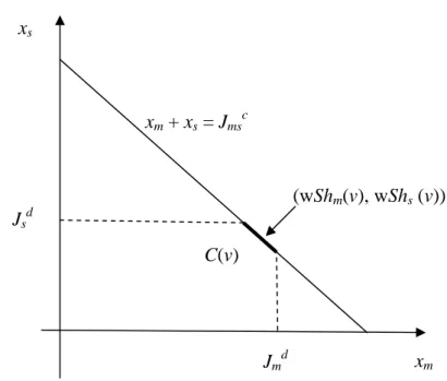
First, we introduce the concept of core (Gillies (1959)). In our model the core of supply chain game v is defined as follows:

} ,

, :

{ )

(v x ^{m,s} x_m x_s J_ms^c x_m J_m^d x_s J_s^d

C = ∈ℜ + = ≤ ≤ ,

where x_m and x_s are coordinates belonging to the manufacturer and the supplier respectively.

The core can be described as it consists of allocations of the total cost of the centralized model such that none of the players can be better off by leaving the centralized model, by stopping cooperation, that is, the core consists of stable (robust) allocations of the costs. It is easy to see that in this model the core is not empty, that is, there is a stable allocation of the costs.

In our model the core has the disadvantage that generally it consists of many points, that is, it is a map-valued solution. Therefore, the following natural question comes up: How can we pick up only one point as a solution? Next we consider a point-valued solution.

Let ω_m,ω_s ≥0 such that ω₁+ω₂ =1^{, then} ωm ^and ωs are called the weights of the manufacturer and the supplier respectively. These weighs can be interpreted as the exogenously given “bargaining powers” of the players.

Shapley (1953) introduced the following point-valued solution concept: The weighted Shapley value of the manufacturer and the supplier respectively in supply chain game v

(

^{msc sd}

)

m d m m

m J J J

v

wSh^{( )} =⁽¹−ω ⁾ +ω − ^,

and

(

^{msc md}

)

s d s s

s J J J

v

wSh = −ω +ω −

2 )1 1 ( )

( .

The weighted Shapley value can be interpreted as it is an adjusted (by the weights) expected value of the given player’s marginal contribution. In other words, e.g. the manufacturer’s weighted Shapley value is the expected value with the distribution

(

(1−ωm),ωm

)

of the manufacturer’s marginal contribution to the cost of the two coalitions not containing her, to the empty collation (J ) and to coalition }_m^d {s (J_ms^c −J_s^d).

In the symmetric case, when the two players have equal power, that is,

2

= 1

= s

m ω

ω ^,

) (v

wSh_m and wSh_s(v) are the so called Shapley value of the manufacturer and the supplier respectively in game v.

Next we show that in our model the Shapley solution is in the core, hence it is a real refinement of this map-valued solution concept.

Lemma 8 For any supply chain game v

(

^wSh(^v)m,^wSh(^v)s

) ( )

∈^{C v} .

Proof. Let (ω_m,ω_s) be an arbitrary weight system. Take the manufacturer first: Lemma 4 implies that

d m m d m m d

s c ms m d m m

m J J J J J

v

wSh( ) =(1−ω ) +ω ( − )≤(1−ω ) +ω , that is, wSh(v)_m ≤J^d_m. In a similar way we can see that wSh(v)_s ≤J_s^d .

Finally, it is obvious that wSh(v)_m +wSh(v)_s = J_ms^c (see e.g. Shapley (1953)).  5 A numerical example

Take the following parameters and cost functions in problems (1)-(2), (3)-(4) and (5)-(8), as in Table 1.

Table 1. Parameter specification for the example

In the following we solve the decentralized and the centralized problem.

5.1 The solution of the decentralized problem

The decentralized problem is a hierarchical production planning problem. First the manufacturer solves her planning problem, then the optimal ordering policy is forwarded to the supplier. Finally, the supplier optimizes her own relevant costs based on the known ordering policy of the manufacturer.

The problem of the manufacturer is as follows:

[ ] [

^{( ) 1}

]

^min

2 5 1 . 0 ) 2 (

5 2

0

2

2 →







 − + −

=

∫

^{I t P t dt}

J_{m m m}

s.t.

5 0

, 25 . 0 ) 0 ( , 2 ) sin(

) ( )

(t =P t − t − I = ≤t≤

I&_{m m m}

The optimal solution can be determined with help of Lemma 2, because the optimal inventory level and production rate are positive. Let the optimal the optimal solution be functions P_m^d(⋅) and I_m^d(⋅).

The minimal cost of the manufacturer is 4.604 units, that is, Jm^d =4.604.

Description Data

Length of planning horizon: T 5

Demand rates: S(t) sin(t)+2

Delay of the supply: τ ^0.5

Manufacturing rate goal level: Pm(⋅) ^1.0

Supply rate goal level: P_s(⋅) ^0.85

Inventory size goal level in manufacturing store: Im(⋅) ^0.5

Inventory size goal level in supply store: I_s(⋅) ^0.3

Initial inventory level in manufacturing store: I_m(0) ^0.25

Initial inventory level in manufacturing store: I_s(0) ^0.5

Manufacturing cost coefficient: c_m 1.0

Supply cost coefficient: c_s 0.5

Inventory holding cost coefficient in manufacturing store: h_m 2

Inventory holding cost coefficient in supply store: h_s 1

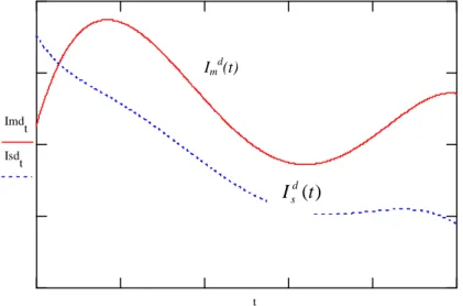
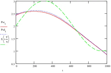
Figure 2. Optimal manufacturing and supply rates for the decentralized models

Psct Psdt

S tT n .

t

In the next step we solve the problem of the supplier, where the manufacturer’s ordering policy P_m^d(⋅) is given:

[ ] [

^{( ) 0.85}

]

^min

2 5 . 3 0 . 0 ) 2 (

5 1

0

2

2 →







 − + −

=

∫

^{I t P t dt}

J_{s s s}

s.t.

5 0

, 5 . 0 ) 0 ( ), ( ) ( )

(t =P t −P t I = ≤t≤

I&_{s s m}^d _s

The optimal solution for the supplier is functions Ps^d(⋅) and Is^d(⋅), applying the results of Lemma 4.

The optimal production rates and inventory levels are shown in Figures 2 and 3.

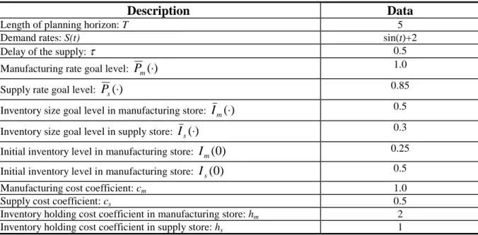
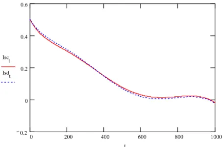
Figure 3. Optimal manufacturing and supply inventory levels for the decentralized models

Imdt Isdt

t

P_m^d(t)

) (t P_s^d

S(t)

Imd

(t)

) (t I_s^d

The minimal cost of the supplier is 2.335 units, that is, Js^d =2.335. The total cost of manufacturer and supplier is 6.939 units in this decentralized strategy of the supply chain, that is J_m^d +J_s^d =6.939.

5.2 The solution of the centralized problem

In the following we solve the centralized problem:

[ ] [ ] [ ] [

^{( ) 0.85}

]

^min

2 5 . 3 0 . 0 ) 2 ( 1 1 ) 2 ( 5 1 . 0 ) 2 (

5 2

0

2 2

2

2 →







 − + − + − + −

=

∫

^{I t P t I t P t dt}

J_{ms m m s s}

s.t.

5 0 , 2 ) sin(

) ( )

(t =P t − t − ≤t≤

I&_{m m}

5 0 ), ( ) ( )

(t =P t −P t ≤t≤

I&_{s s m}



 



=









5 . 0

25 . 0 ) 0 (

) 0 (

s m

I I

The optimal solution of this problem is given after the solution of the following differential equation (see (9)):





















−

−

−

− +





















⋅





















−

= −





















6 . 0

7 . 0 0

2 ) sin(

) (

) (

) (

) (

0 0 2 0

0 0 1 2

1 1 0 0

0 1 0 0

) (

) (

) (

)

( t

t P

t P

t I

t I

t P

t P

t I

t I

c s

c m c s c m

c s

c m c s c m

&

&

&

&

(9)

with initial and terminal conditions







=









5 . 0

25 . 0 ) 0 (

) 0 (

s m

I

I ,

and

85 . . 0

1 )

( )

( 



 



=











 T P

T P

c s

c m

The optimal production rates and inventory levels are shown in Figures 4 and 5.