Ultrasound Image Modelling and Resolution Enhancement
Akos Makra ´
Supervisor: Dr. Mikl´ os Gy¨ ongy
P´ azm´ any P´ eter Catholic University
Faculty of Information Technology and Bionics Tam´ as Roska Doctoral School of Sciences and Technology
A thesis submitted for the degree of Doctor of Philosophy
2020
Contents
Glossary . . . viii
0.1 Declaration of original work used . . . xiv
1 Introduction 1 1.1 Motivation . . . 1
1.1.1 Relevance of ultrasound imaging . . . 1
1.1.2 Relevance of validation of image formation models . . . 2
1.1.3 Relevance of resolution enhancement . . . 3
1.2 Overview of current thesis . . . 4
2 Theory 5 2.1 Basics of ultrasound imaging . . . 5
2.1.1 Transducer . . . 6
2.1.2 Beam parameters of spherically focussed transducers . . . 8
2.1.3 Axial and lateral resolution . . . 10
2.1.4 Ultrasound imaging modes . . . 13
2.2 Theory of ultrasound image formation . . . 16
2.2.1 Overview . . . 16
2.2.2 Governing equations of acoustics . . . 17
2.2.3 The homogeneous linear wave equation . . . 22
2.2.4 The inhomogeneous linear wave equation . . . 23
2.2.5 Scattering . . . 25
2.2.6 Complete shift-variant convolution model of US imaging . . . 26
2.2.7 Shift-invariant convolution model . . . 28
2.3 Theory of resolution enhancement . . . 29
2.3.1 Mathematical formulation . . . 29
2.3.2 PSF estimation . . . 30
2.3.3 Classical deconvolution-based methods . . . 32
2.3.4 Cost function minimization . . . 34
2.3.5 Deep learning . . . 35
2.3.6 US specific methods . . . 38
3 Experimental validation of ultrasound image formation 44 3.1 Introduction . . . 44
3.2 Methods . . . 46
3.2.1 SF estimation . . . 46
3.2.2 PSF estimation . . . 47
3.2.3 Evaluation of simulation accuracy . . . 48
3.2.4 Sources of error . . . 48
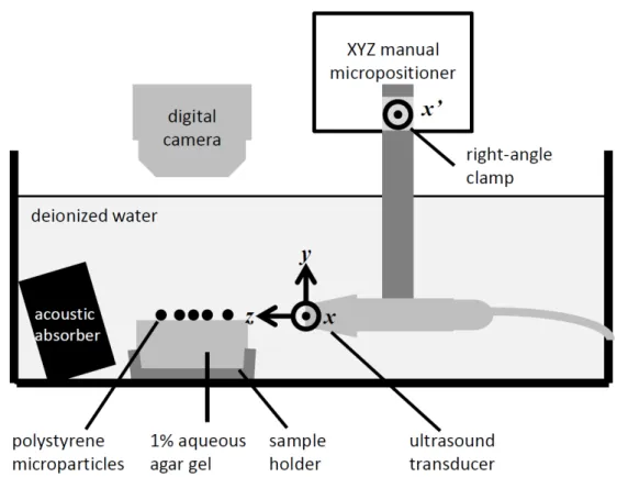
3.2.5 Generation of co-aligned US image and SF . . . 49
3.2.6 Estimation of the PSF . . . 53
3.2.7 Convolution-based ultrasound simulations . . . 54
3.3 Results and discussion . . . 56
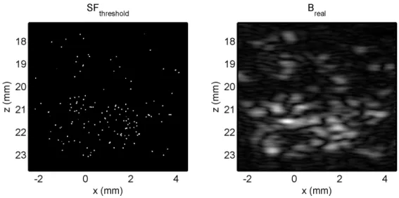
3.3.1 Generation and registration of ultrasound image with scatter- ing function . . . 56
3.3.2 Estimation of PSF . . . 56
3.3.3 Convolution-based ultrasound simulations . . . 57
3.4 Conclusions . . . 62
4 Resolution enhancement of high-resolution B-mode images using axial processing 65 4.1 Introduction . . . 65
4.2 Methods . . . 66
4.2.1 Simulations . . . 66
4.2.2 Agar-graphite phantom . . . 66
4.2.3 Skin examination . . . 66
4.2.4 Deconvolution . . . 67
4.2.5 Scaled RAMP filtering in the frequency domain . . . 67
4.2.6 Resolution estimation . . . 68
4.3 Results and discussion . . . 68
4.3.1 Simulations . . . 68
4.3.2 Agar-graphite phantom . . . 69
4.3.3 Skin examination . . . 70
4.3.4 Resolution estimation . . . 71
4.4 Conclusions . . . 73
5 Resolution enhancement of C-mode SAM images 74 5.1 Introduction . . . 74
5.2 Methods . . . 75
5.2.1 Experiment . . . 76
5.2.2 Image resolution enhancement . . . 77
5.2.3 Resolution metrics . . . 80
5.3 Results and discussion . . . 81
5.4 Conclusions . . . 91
6 Summarizing conclusions 92
List of Figures
2.1 Sound field of a single-element transducer . . . 9
2.2 Full-width at half maximum . . . 10
2.3 Lateral resolution . . . 12
2.4 Axial resolution . . . 13
2.5 A conventional A-line . . . 14
2.6 Schematic of a SAM system . . . 15
2.7 Block diagram of US image formation . . . 16
2.8 Pressure and density scalar fields . . . 18
2.9 Continuity equation . . . 20
2.10 Geometry to determine transmit-receive response . . . 27
2.11 The transmit and receive responses in time-domain . . . 27
2.12 Schematic of a neuron and its corresponding mathematical model . . 35
2.13 Network layers . . . 36
2.14 Convolutional Neural Network . . . 37
2.15 Field II-simulated 2-D PSF of a single-element transducer and its corresponding lateral spectral distribution . . . 42
3.1 Schematic diagram of experimental setup . . . 49
3.2 Steps in estimating the SF of the polystyrene scatterers from a macropho- tograph . . . 52 3.3 Alignment of estimated SF with experimentally obtained B-mode image 56 3.4 Comparison of different estimates of the PSF of the imaging system . 57
3.5 Spatial sensitivity of the coefficients of determination R2 for the RF and envelope (B-mode) data between real and simulated ultrasound images . . . 58 3.6 Comparison between the real ultrasound (left) and simulated ultra-
sound images computed using three different estimates of the SF (Fig. 3.2) . . . 59 3.7 Comparison between the real ultrasound image (first column) and
simulated ultrasound images computed using six different estimates of the PSF (Fig. 3.4) . . . 59 3.8 Comparison between real ultrasound images and a simulated image . 60 3.9 Comparison of two real ultrasound images, one generated without,
the other with dynamic receive apodization . . . 61 3.10 Estimation of the spatial variation of the coefficients of determination
R2 for both the RF images I and B-mode images B . . . 61 4.1 Resolution enhancement on a sparsely populated area (simulation)
using deconvolution . . . 68 4.2 Resolution enhancement on a densely populated area (simulation)
using deconvolution . . . 69 4.3 Axial and lateral mean AC curves of the envelope images (sparse area) 69 4.4 Axial and lateral mean AC curves of the envelope images (dense area) 70 4.5 Resolution enhancement on an agar-graphite phantom B-mode US
image using axial deconvolution . . . 70 4.6 Axial and lateral mean AC curves of the envelope images (tissue-
mimicking phantom) . . . 71 4.7 Resolution enhancement of a skin (nevus) B-mode image using de-
convolution . . . 71 4.8 Axial and lateral mean AC curves of the envelope images (clinical
skin image) . . . 72 5.1 Depiction of the four-layered convolutional network . . . 80
5.2 Co-registered 180- and 316-MHz C-scan SAM image pairs of rat and mouse brain sections . . . 83 5.3 Results of the different resolution enhancement methods on the test
image . . . 84 5.4 Representative sample from Fig. 5.3 (top left marked area) . . . 85 5.5 Representative sample from Fig. 5.3 (marked area in the middle) . . . 86 5.6 Representative sample from Fig. 5.3 (bottom right marked area) . . . 87 5.7 NRMSE values of the different image resolution enhancement methods 88 5.8 PSNR values of the different image resolution enhancement methods . 88
List of Tables
3.1 Short summary of the PSF and SF estimates. . . 54 4.1 FWHM values of the AC functions . . . 72 5.1 Properties of the transducers used during the experiment and PSF
simulation. . . 76 5.2 Estimated resolution of the C-scan images of Figs. 5.4 – 5.6. . . 89
Glossary
Notation Description Page
List
. element-wise multiplication 29
⊗ correlation operator 33
∇ nabla operator 19
∇2 the Laplacian, ∇2 =∇ · ∇ 22
Π (.) rectangular function 39
III (.) Dirac comb (Shah function) 39
F {.} Fourier transform 29
F−1{.} inverse Fourier transform 47
k.k norm 34
] phase of the complex functions 32
∆κ deviation from mean compressibility at equilibrium 23
∆ρ deviation from mean density at equilibrium 23
Λ appropriate weight for a desired sparsity 34
β bulk modulus, inverse of compressibilityκ 21
γ p-value for the lp norm, 0≤p≤2 34
κt total compressibility 23
κv equilibrium compressibility 23
κ compressibility 21
λ wavelength 8
φ(r, t) scattered field 24
ψ(.) Lucy–Richardson function 33
ρ0 mean density at equilibrium 18
ρt total density 18
ρv equilibrium density 23
ρ density 26
σ variance of the noise 33
Notation Description Page List
τ spatial pulse length 12
σ2u variance of all the pixel values of image u 48
a scaling term 48
AC autocorrelation 44
ADMM alternating direction method of multipliers 34
ANN artificial neural network 35
ARMA autoregressive moving average 31
b bias 35
Breal real B-mode US image 48
Bsim simulated B-mode US image 48
BD beam diameter 10
BW bandwidth 39
c speed of sound 8
cycles# number of cycles in the pulse 12
CNN convolutional neural network 36
dx interpixel-distance of macro photograph 52
D diameter of the aperture 8
DL deep learning 35
ei input voltage 27
E additive error term 48
f frequency 8
f(t) total pressure acting on the transducer 27
f(z) activation function 35
f# f-number 11
FL focal length 11
FWHM full-width at half maximum 10
Notation Description Page List
g optimal filter 32
G Fourier transform of g 32
h transfer function (PSF) 29
hmp 1-D minimum-phase estimate ofh 30
hpe geometric response of the ultrasound transducer 41 hs pressure impulse response of the scatterer 27
ht velocity potential impulse response 27
H Fourier transform of transfer function h 29
H∗ complex conjugate of H 33
i(z) backscattered signal in the axial direction 38
I(u) Fourier transform of i(z) 39
Ireal real US image (post-beamformed RF) 48
Isim simulated US image 48
J cost function 34
ML machine learning 35
MSE mean squared error 32
n noise 29
˜
n normal unit vector 19
N near field distance 8
Fourier transform of the noisen 29
NRMSE normalized root mean square error 80
NSR noise-to-signal ratio, inverse of SNR 33
p (acoustic) pressure 17
p(z) PSF in the axial direction 38
p0 mean pressure at equilibrium 18
pi incident presssure 25
Notation Description Page List
pr pressure on the transducer surface 27
ps scattered presssure 25
pt total pressure 18
P(u) Fourier transform of p(z) 39
PSF point-spread function 28
PSFdata data-based PSF 53
PSFdeconvolution deconvolution-based PSF 53
PSFest estimated PSF 48
PSFFieldII Field II-based PSF 53
PSNR peak signal-to-noise ratio (peak SNR) 81
r position vector 17
r0 location of acoustical disturbance 25
r0 location of single scatterer 26
rr location of transducer surface 27
R reflection coefficient 26
R(f) RAMP function (function of frequency) 67
R2 coefficient of determination 46
RA axial resolution 11
R2B R2 between the simulated and real B-mode US images 48 R2I R2 between the simulated and real US images 48
RL lateral resolution 11
RAMP frequency-weighted axial filtering 67
RF radio-frequency 14
s distance 14
s(z) SF in the axial direction 38
S surface area 19
Notation Description Page List
S(u) Fourier transform of s(z) 39
Skernel size of the kernel 38
Slim(u) band-limited Slim(u) 39
SN power spectrum density of the noise 33
Sr area of the receiver the transducer 27
St area of the transmit the transducer 27
SX power spectrum density of the signal 33
SAM scanning acoustic microscopy 15
SBE step-based estimation 77
SF scattering/scatterer function 2
SFest estimated SF 48
SFpoints point-based SF from SFproject 51
SFproject projection-based SF from SFthreshold 51
SFthreshold threshold-based SF 51
SNR signal-to-noise ratio, inverse of NSR 42
SR super-resolution 3
t time 17
tp elapsed time between the emitted pulse and detected echo 14
TV total variation 34
u angular frequency 39
u0 central frequency 39
US ultrasound 1
v particle velocity 17
vpe electric response of the ultrasound transducer 41
V volume 19
w0 weight parameter 35
Notation Description Page List wrδ electromechanical response of the receive transducer 27 wtδ electromechanical response of the transmit transducer 27
x lateral distance 5
underlying structure (SF) 29
ˆ
x estimated input 32
x0 neuron input 35
ˆ
xk the estimate ofx after k number of iterations 33 X Fourier transform of underlying structure x 29
Xˆ Fourier transform of estimated input ˆx 32
y elevation distance 5
observed image 29
ymax maximum value of image y 81
ymin minimum value of imagey 81
Y Fourier transform of observed image y 29
z axial distance 6
Z acoustic impedance 26
Z1 acoustic impedance of the first medium 26
Z2 acoustic impedance of the second medium 26
ZP zero-phase (estimate) 43
0.1 Declaration of original work used
This section introduces the main references of the current thesis. In Chapter 1, Section 1.1.2 is based on [Au1], Section 1.1.3 is based on [Au2, Au3]. In Chapter 2, Section 2.1 is based on the Master’s Thesis of the author [Au4], Section 2.2 is based primarily on the Bachelor’s Thesis of the author [Au1], in which Section 2.2.7 is based on [Th1]. Furthermore, Sections 2.3.1, 2.3.2 and 2.3.4 are based on [1] [Au2], and Section 2.3.6 is based on [Au5]. Chapter 3 is based on [Th1], Chapter 4 is based on [Th2], and Chapter 5 is based on [Th3].
Further references, which are mostly independent of the author, are provided in the appropriate (sub)sections. To facilitate differentiation, pictures taken verbatim from the publications of the author are indicated by a standalone citation at the end of the figure caption, whereas modified/adapted or images taken verbatim from other sources are annotated in a normal manner.
Chapter 1 Introduction
1.1 Motivation
1.1.1 Relevance of ultrasound imaging
Diagnostic ultrasound has been in use for 60 years now and it has become one of the most popular medical imaging methods nowadays. Diagnostic ultrasound imaging commonly utilizes frequencies in the range of 3–20 MHz. The use of higher frequencies limits the depth of penetration, however it also increases resolution.
Recently, ultrasound (US) has been actively used not only for medical diagnos- tic purposes [2–4], but also for high-intensity focal beam surgery to produce precise and selective damage to tissues [5–7], biometric recognition [8], non-destructive test- ing [9–19], and has many applications in the food industry [20–23] among others.
Its wide range of applications stems from its numerous advantages such as cost- effectiveness, portability, and using non-ionizing radiation compared to many other procedures such as X-ray, CT or PET, all of which are using potentially harmful ra- diation. On the other hand, the interpretation of US images is still quite a subjective task despite the numerous quantitative US studies [24–33].
The connection between the fine microscopic structure of tissues and the re- sulting US image is at present not fully understood, which further motivates the development and the importance of validating image formation models.
1.1.2 Relevance of validation of image formation models
Interpretation of US images is quite a subjective task, so the mapping of the var- ious histological pathologies is an empirical (and implicit) procedure for the radiol- ogist experts. There are many theoretical models to describe US imaging, however, there is little research to validate these models. The following paragraphs attempt to categorize these approaches.
First, for US imaging to occur, US needs to propagate to the scatterers in ques- tion, then scattering of the incident wave must occur, and the scattered wave must propagate back to the transducer. The difference lies in how these phenomena are treated in US imaging models.
Propagation is usually considered to be linear, which is based on the assumption that the deviations in pressure and density that support the propagation of the wave (for more details see Section 2.2.4) are small relative to the mean pressure and density. If the medium is homogeneous, the waves travel through unimpeded;
however, any degree of inhomogeneity causes ultrasound scattering, which arises from perturbations in density and compressibility [34]. Considering the backscatter of ultrasound in the direction of the original incident wave (180◦ scattering), the scattering function (SF) in terms of density and compressibility may be reduced to a SF (or alternatively, tissue reflectivity function) expressing relative changes in acoustic impedance, which is consistent with the 1-D model of wave reflection [35, 36] [37, pp. 304–306]. Other authors have opted to express this scattering function in terms of changes in the bulk modulus [38].
Another issue concerning modeling is the nature of the scattering. Most models neglect multiple scattering and assume that the scattered field is generated only by the incident field, an assumption known as the Born approximation (see Sec- tion 2.2.5). However, there is a conceptual split in research that treats the scatter- ing medium as consisting of discrete scatterers [34, 38] and those that regard it as a continuously varying acoustic maps [39].
Another simplification is to assume the impulse response of the scatterers spa- tially invariant [40], which means that the position of the scatterer relative to the US transducer is irrelevant in the terms of impulse of the scattering. This assumption
is called shift-invariance. For more detail about the validity of this simplification, the reader is directed to [41] and Chapter 4.
If as a first step, it would be possible to validate an image formation model with simple, inanimate scatterers, it would open the way toward exploring the relationship between histology and US images.
1.1.3 Relevance of resolution enhancement
Imaging modalities of any kind have a theoretical limit on their feasible resolu- tion. The objective of the super-resolution (SR) algorithms is to break this boundary, thereby obtaining an image of higher quality with the same physical setup.
There has always been a great demand for producing images with better and bet- ter resolution, either by creating a better physical setup, or using post-processing techniques, whether it is about security cameras [42–44], satellites [45–50], profes- sional photography [42, 51–53] or even the HUBBLE space telescope [54–57]. The same rules apply for medical purposes: the higher the resolution of an image, the more precise the diagnosis.
Concerning software-based methods for enhancing image resolution, the algo- rithm can be used either on sub-pixel-shifted frames by stacking them, or as a post-processing step where even one frame can be satisfactory. The use of SR tech- niques provides the possibility of receiving a more detailed image at a lower cost compared to the expensive and time-consuming process of building a new hardware capable of delivering the same quality.
Nevertheless, along with other imaging modalities (such as MR, CT or light microscopy) its resolution is heavily dependent on the wavelength (higher frequency, thus shorter wavelength leads to better resolution), which in the case of sound is a lot poorer than that of light or X-ray. The transducer and its frequency also determine the penetration depth (the higher the frequency, the smaller the mentioned depth is) [58, p. 116]. To be able to examine deeper layers of the medium, lower frequencies should be used, which, however, decreases the resolution.
Taking into account the benefits of US imaging it would be worthwhile if the image resolution and signal-to-noise quality could be improved by post-processing
methods. This work is concentrated around US images; however, the algorithms to be presented can be adapted to other imaging modalities as well.
1.2 Overview of current thesis
In this section a brief overview of the current thesis is given.
In Chapter 2, the theoretical basis of ultrasound image formation and resolution enhancement is described. In Section 2.2, the theoretical background of acoustics and the basic concepts regarding US are introduced, including the shift-invariant convolution model. In Section 2.3, the mathematical background of resolution en- hancement is provided. Further in this section, the classical deconvolution tech- niques used for image resolution enhancement are described in Section 2.3.3, with cost function minimization in Section 2.3.4. The theoretical background of deep learning is introduced in Section 2.3.5. Last, the current US specific resolution en- hancement methods are discussed in Section 2.3.6, with an emphasis on equivalent scatterers and axial processing.
The next chapters introduce the scientific work of the author. In Chapter 3, a method to experimentally assess the accuracy of the previously described shift- invariant convolution model (see Section 2.2.7) is presented. In Chapter 4, the resolution enhancement of ultrasound B-mode images using deconvolution (see Sec- tion 2.3.3) and axial processing (see Section 2.3.6) is presented, whereas Chapter 5 demonstrates the resolution enhancement of ultrasound C-scan images using deep learning (see Section 2.3.5).
In Chapter 6, a summary is given about the new scientific results of the author in the form of thesis points.
Chapter 2 Theory
2.1 Basics of ultrasound imaging
The aim of the current section is to provide the reader with the basics of ultra- sound imaging and introduce the main concepts regarding the topics covered in this thesis.
Mechanical waves with frequencies higher than 20 kHz are called ultrasound. Its propagation results in a periodic change of pressure in space and time. Ultrasonic diagnostics take advantage mainly of the fact that ultrasound waves are reflected from different interfaces in the medium: the elapsed time and the intensity of the reflection can provide a good estimate about the physical properties of the examined medium.
As with any imaging modality, there are a set of different parameters which to- gether adequately describe the system. In general, these parameters are not indepen- dent of each other, and the choice of parameters greatly determines the application area. A simple example is when the central frequency of the transducer is increased, which (assuming an increase in bandwidth) leads to greater resolution but at the same time decreases penetration depth and hence more superficial examination of the tissue. Given the above consideration, it is crucial to have a clear understanding of the basics of image formation and to be aware of the connections and trade-offs between the system parameters.
Conventionally, the lateral, elevation, and axial directions are denoted by x, y,
and z, respectively, unless otherwise noted.
The following sections (Sections 2.1.1 to 2.1.4) are primarily based on the fol- lowing sources [37, 58, 59] unless otherwise annotated.
2.1.1 Transducer
A transducer is a device capable of transforming energy from one form to an another. In the case of US, it converts the electrical energy into mechanical pressure waves and vica versa, by utilizing the inverse and direct piezoelectric effects (discov- ered by the Curie brothers in 1880 [60] [58, p. 3]), respectively. It has two different modes, namely transmit and receive. During transmission mode it emits (a series of) sound waves into the body by converting electrical energy to pressure vibrations (inverse piezoelectric effect). In receive mode it captures the backscattered sound waves and interprets those as electrical signals (direct piezoelectric effect).
The fundamental part of the transducer is the piezoelectric element itself. In general, it is made of a crystal-like material like tourmaline, quartz, topaz or cane sugar [61]; however, synthetic materials, like poly-vinylidene fluoride [62] are capable of producing the piezoelectric effect as well.
Since the discovery of the piezoelectric effect many forms of the transducer have been invented, each of them suitable for different tasks. In this section the main types of transducers will be introduced.
Transducer types
1. Single-element transducers: The simplest form of transducers are made of a single element. For focusing, two methods may be used. One of them focuses the beam using an acoustic lens, which for instance can be made of plastic, epoxy, liquid or rubber [63]. The other method is to press the element itself into a curved shape [64]. Since single-element transducers only have a fixed focus, in order to capture an image manual scanning has to be performed. Note that even a so-called unfocussed (flat-surface) single-element transducer has a natural focus, which is defined by Eq. (2.1). In addition, the lateral resolution
changes with depth, which can lead to a false impression of inhomogeneity even in the case of a homogeneous sample.
2. Linear array transducers: The second main form of transducers is the linear array. It contains a line of elements (for instance 320 pieces, spaced over an aperture of 56 mm [65]). The smaller the face of the transducer, the more divergent the beam will become during propagation. In order to decrease this divergence, a subset of the elements (8-16) is selected and pulsed simultane- ously. For the next line the neighbouring subgroup will be activated (shifting the previous elements by one) and so on. However, due to the shifting sub- aperture, the physical footprint of this arrangement is sometimes too large to scan through relatively small acoustic windows (such as in imaging the heart through the ribs).
3. Phased array transducers: In the phased array, the elements are again placed in a row like in the case of the linear array. However, this time, all the ele- ments are excited together but with small time-delays, needing independent delay circuits. This manner of emission of sound waves results in a curved propagating wavefront. By changing the length of delays, the beam can be steered into various directions and with different focal lengths. When receiv- ing the signal, the same delay factors can be used in order to have dynamic focusing, meaning all points along the z-axis will be in focus. Since there is no shifting sub-aperture, the footprint of the transducer can be as small as 2 cm.
More generally, if the elements are arranged on a planar grid, the beam can be steered in three dimensions, resulting in 3D ultrasonic imaging. By combining linear and phased arrays, the reduction of beam-divergence and focusing can be accomplished at the same time.
4. Annular array transducers: The last common transducer type to be discussed in this introduction is the annular array. In this case the elements are arranged as a set of concentric rings, possibly evenly placing them at different heights, giving a spherical curvature to the array. However, this curvature can be also achieved by activating the circle-elements with time-delays. It also records
a single line at a time as single-element transducers, but gives a better and possibly changeable focus, and greater depth of field as well. Effectively, a large number of fixed-curvature spherical transducers can be placed farther away, thus they can be used with higher frequency. The limit which needs to be considered when placing the elements is the effect of grating lobes, which can be overcome by creating the transducer elements to be smaller than half of the used wavelength. In phased arrays, the creation of such small electrical circuits is always a challenge; however, annular arrays do not suffer from this restriction.
2.1.2 Beam parameters of spherically focussed transducers
Spatial distribution of the ultrasound field
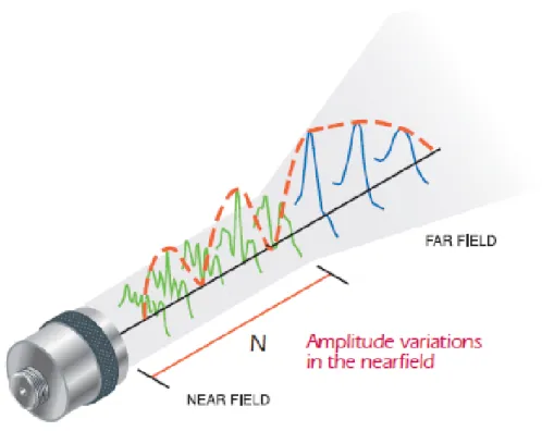
The spatial distribution of the US field (otherwise referred to as the ultrasound beam) is generated as a result of the inverse piezoelectric effect, when applied voltage is transformed into a periodically varying pressure (sound) wave. The beam can be divided into two regions: near field (Fresnel zone) and far field (Fraunhoffer zone). Figure 2.1 shows that in the near field the pressure intensity reaches multiple local minima and maxima and ends in a last, global maximum, called near field distance. The distance at which the far field begins can be calculated by the following formula [59, p. 43]:
N = D2f 4c = D2
4λ , (2.1)
where N means the near field distance, D is the diameter of the aperture, f is the frequency, c stands for the propagating speed of sound in the medium, and λ annotates the wavelength. It is important to note that the near field is the same for both unfocussed and geometrically focussed transducers. However, the focal length will differ, meaning that the focal length will coincide with the near field distance for an unfocussed transducer.
In the far field the beam becomes divergent, causing the lateral resolution to heavily decrease. Geometrically focussed transducers with help of an acoustic lens will cause the beam width to decrease at a certain distance (focal length) from the
Figure 2.1: Sound field of a single-element transducer. The emitted beam can be divided into two parts: the near field (Fresnel zone) and the far field (Fraunhoffer zone). The near field starts directly after the transducer surface, where the amplitude of the pressure wave reaches several local minima and maxima, and ends in a last, global maximum. The location of the last point defines the near field distance (which in the case of geometrically unfocussed transducers is the same as the focal length), and is annotated by N in the figure. Beyond the near field distance begins the far field, where the intensity of the sound wave decreases progressively to zero due to the divergent nature of the beam. Picture taken from [59, p. 43].
transducer, which distance, as a rule of thumb, is approximately half of the radius of the curvature. As a result, at the focal length the lateral resolution will improve, as well as the extent of divergence of the beam in the far field, but the depth of field will be decreased.
In addition to the relatively simple concept of a transmitted beam, an analogous concept exists for the so-called receive beam, which is the spatial distribution of the receive sensitivity of the ultrasound transducer. Where the same transducer is used for transmit and receive, the transmit and the receive beams can generally be considered to have the same shape.
2.1.3 Axial and lateral resolution
The beam diameter (BD), which is equivalent and often referred to as beam width, plays an important role when it comes to the sensitivity of a transducer. The beam consists of side lobes and a main lobe, which together are considered as the beam. Side lobes are essentially off-axis energies which can lead to different artefacts and are dependent on many factors such as the frequency, element spacing, number of elements and bandwidth. At the point of interest the smaller this diameter is the more energy is concentrated onto that point, which means the more energy will be reflected, resulting in a higher lateral resolution.
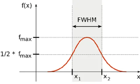
To define beam width, it is needed to define the full-width at half maximum (FWHM) [37, p. 173]. Considering a distribution function (such as pressure am- plitude ∆p(x)), as it can be seen in Fig. 2.2, around its maximum value such an interval can be found along the x-axis, where the value of the function is higher or equal than the half of the maximum value. In the literature, generally the -6 dB pulse-echo criteria is used, which is an equivalent form due to the fact that it de- scribes such a relationship where the voltage amplitude of the output is half of the input. This interval along the x-axis defines the so called FWHM.
Figure 2.2: Full-width at half maximum. Considering a distribution function, the so-called full- width at half maximum means such an interval along the x-axis, where the value of the function is equal or higher than the half of the maximum. Note that f(x) represents a voltage-like function, such as pressure amplitude∆p(x). Picture taken from [66].
TheBDvaries along the main lobe axis, as it is typically wide (in a perpendicular plane to the propagation direction) in the near and far fields and is the smallest at the focal length. The -6 dB pulse-echo BD at the focal length can be estimated, taking into account the FWHM definition and the Sparrow criterion [67, p. 189], as follows [59, p. 43]:
BD= 1.02λ· FL
D = 1.02λ·f#, (2.2)
where FL stands for the focal length, D is the diameter of the aperture, and f# is the f-number of the transducer.
On one hand, as it has been described above, the BD will determine the lat- eral resolution of the system (the lateral size of the received signal), as shown in Fig. 2.3 a). On the other hand, this resolution describes what is the smallest dis- tance between two scatterers – in a perpendicular plane to the propagation – which can still be distinguished (see Fig. 2.3 b)). It essentially means when two scatterers are in the same plane and both of them are inside the main lobe, they cannot be distinguished; however, if one of them is located outside, the system is capable of identifying them as two different structures.
The lateral resolution RL can also be derived from Rayleigh scattering, when a scatterer is much smaller compared to the wavelength. In this case the lateral resolution can be estimated (taking into account the Rayleigh criterion [67, p. 187]) as follows [37, p. 173]:
RL = 1.22λ· FL
D = 1.22λ·f#, (2.3)
where the multiplication factor of 1.22 is present due to the Bessel functions [37, p. 173] and Rayleigh criterion [67, p. 187].
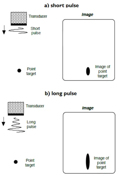
The axial resolutionRA is also an important parameter of an imaging system. It describes what is the smallest distance between two scatterers located parallel to the beam, which can still be distinguished (see Fig. 2.4). It is determined by the spatial pulse length, which is the number of cycles in the pulse multiplied by the wavelength of the propagating pressure wave, and can be estimated as follows [37, p. 511]:
RA= 1
2λ·cycles#= 1
2τ , (2.4)
Figure 2.3: Lateral resolution. Figure 2.3 a) shows that how scatterers at different locations on the main axis would be present in an ultrasound image with the given beam profile. The farther the scatterers are from the focal length where theBDis the smallest, the laterally distorted they appear in the actual ultrasound image. In addition, in Fig. 2.3 b) it can be seen when two scatterers are inside the beam in the focal length plane, and in that case they cannot be distinguished from each other as two different scatterers. On the other hand, if one of those scatterers is outside the beam, they will appear in the ultrasound image as different objects. Picture adapted from [68, p. 13].
whereλ is the spatial wavelength, cycles# is the number of cycles in the pulse, and τ represents the spatial pulse length.
Figure 2.4: Axial resolution. The axial resolution is determined mainly by the length of the excita- tion pulse (or the so-called number of cycles parameter). In Figure a) it can be seen that the axial resolution is decent in case of using a short pulse as excitation. Figure b) shows a big amount of axial distortion in case of using a long pulse. Picture adapted from [68, p. 14].
2.1.4 Ultrasound imaging modes
There are different ultrasound imaging modes such as A-mode, B-mode, B-flow, Doppler, Power Doppler, C-mode, or M-mode among others; however, this work is based on the conventional A-mode, B-mode and C-mode imaging. This section describes these methods.
Figure 2.5: A conventional A-line. The first 5μs shows an artefact of the imaging system due to the constant high frequency switch between transmit and receive modes. Around 32 μs a reflection can be observed from the boundary of two media having different physical properties. Picture taken from [Au4].
A-mode
The so-called A-mode means Amplitude-mode and is the simplest of all modes.
It corresponds to the conventional oscilloscope display, when an emitted pulse is returned as an echo due to local inhomogeneities, and it is displayed as a function in a time-amplitude (or distance-amplitude) plane, where a higher amplitude means a greater acoustic impedance difference between the boundaries. Such an A-line can be seen in Fig. 2.5. Other sources refer to A-lines after taking the envelope of the post-beamformed radio-frequency (RF) signal. The distance from the surface of the transducer can be calculated knowing the propagating speed of sound in the medium as follows:
s= c·tp
2 , (2.5)
where s is the distance, c is the speed of sound in the examined medium, and tp stands for the elapsed time between the emitted pulse and detected echo.
B-mode
A B-mode image shows a cross-section plane of the medium, which is parallel to the propagating waves. The so-called B-mode means Brightness-mode and orig-
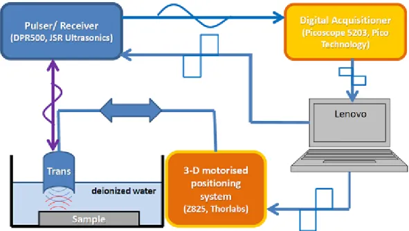
inates from the conventional display of US images, where the higher amplitude of a pulse-echo signal is, the brighter is the image at those areas. An actual B-mode image can be generated using a plethora of different insonification strategies such as focussed beams or diverging-wave transmissions [69]. It is also possible to record equidistant A-lines with a single-element transducer,e.g., by using a scanning acous- tic microscope system (SAM) (see Fig. 2.6), and use the envelope of the amplitude for the visualization to produce a B-mode image. The A-lines can be put next to each other based not only on distance, but time or angle as well.
Figure 2.6: Schematic of a SAM system. During the movement of the transducer the impulse generator (or referred to as pulser) at a certain desired frequency receives a trigger signal, which generates a short electric impulse with a high amplitude. This electrical impulse will be transformed into a sound (pressure) wave, which is (generally) focussed on the surface of the sample. The scattered (reflected) wave will be detected, converted back to electric impulse and will get recorded by the digital acquisitioner. After saving the desired data, the transducer moves to the next position with the help of the micropositioner system. Picture taken from [Au4].
C-mode
C-mode imaging results in such a cross-sectional plane of the examined media, which is normal to the propagating waves (and therefore to the B-mode images). C- mode images are usually generated by a SAM system, where a motorized movement
of a single-element transducer performs a scan over a pre-defined grid (usually in 2- D) and records an A-line at every grid point. Such a system can be seen in Fig. 2.6.
By providing depth information over a 2-D plane the result is a 3-D volumetric data.
Such A-lines can be either integrated over a given window axially or individual planes can be displayed selecting the same depth along every A-line.
One common form of SAM imaging involves taking the integral of the absolute values of A-lines in the axial direction, which is used for the visualization process, resulting in a C-scan image.
2.2 Theory of ultrasound image formation
2.2.1 Overview
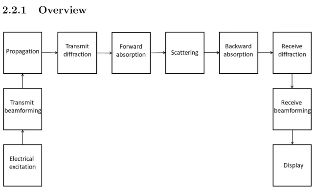
Figure 2.7: Block diagram of US image formation listing the major processes. Image is based on [70, p. 43]
For an ultrasound image to occur, there are many steps which have to be con- sidered during the US image formation. Figure 2.7 lists the major processes. For more comprehensive system details the reader is directed to [70, pp. 43–45].
First, an electrical excitation is used on the transducer. The transmit beam- former by receiving this signal ensures that the appropriately delayed pulses arrive
at the transducer elements. The array elements convert the electrical energy to pressure (sound) waves by utilizing the inverse piezoelectric effect (as mentioned in Section 2.1.1). The propagating waves are undergoing diffraction, absorption, and scattering (both travelling further away and back towards the transducer), during which its energy is decreased (this energy loss can be compensated for). Upon the waves reaching the surface of the transducer, the pressure is going to be converted back to electrical signals, taking into account the appropriate time delays. Before the display, the data can be post-processed with different techniques such as time gain compensation, speckle reduction, envelope detection or log-compression among others, to meet desired needs.
In the following, the physics behind the two most thesis-related processes will be introduced, namely the propagation (see Sections 2.2.2 and 2.2.3) and scattering (see Sections 2.2.4 and 2.2.5). Next, the whole image formation will be described as a shift-variant convolution-model, taking into account certain assumptions (see Section 2.2.6). Last, the shift-invariant convolution model will be introduced (see Section 2.2.7).
2.2.2 Governing equations of acoustics
In this section, the governing equations of acoustics, which are going to lead to the homogeneous acoustic linear wave equation, will be derived using the following sources: [37, Sections 1.3.5 and 5.4] [71, Section 2.1.1] [72, Chapter 2] [73, Chap- ter 1] [74, Section 3.5 and Chapter 16] [34].
Acoustics deals with describing the propagation of mechanical waves through different media. The acoustic wave equation is a second order partial differential equation, which establishes a relation between the acoustic pressure p and particle velocityv as a function of position r and time t.
To obtain a linearized form of the wave equation, it is crucial to use approxima- tions, and further variables need to be defined. First of all, it is assumed that the acoustic pressure and density can be written as
pt(r, t) = p0+p(r, t) (pp0) (2.6)
ρt(r, t) = ρ0+ρ(r, t) (ρ ρ0) (2.7) at any given location r and time t, in whichpt is the total pressure, p0 is the mean pressure at equilibrium, p is the pressure fluctuation caused by the propagating wave, ρt is the total density, ρ0 stands for the mean density at equilibrium and ρ is the density fluctuation induced by the wave. Figure 2.8 illustrates the situ-
Figure 2.8: A volume of fluiddV with the local pressurepand local densityρcan be seen. The local pressure and density variations are generated by an acoustic disturbance (such as a propagating wave through the media). The mean pressure and density at equilibrium are denoted byp0 andρ0, respectively. Picture adapted from [72, p. 6].
ation: there is a fluid volume dV with mean pressure p0 and mean density ρ0 at equilibrium. After any acoustic disturbance local pressure and density fluctuations can be observed, denoted by p and ρ, respectively. Considering these assumptions, the ultrasound waves cause perturbations around the mean density and pressure;
furthermore, these perturbations are assumed to be small. To fully describe the acoustic field, the following three equations are needed to derive in linearized forms:
equation of motion, continuity equation and equation of state.
The equation of motion
The equation of motion is based on Newton’s second law, forming a relationship between the force acting on the fluid particle’s volume and its momentum’s alter- ation. Considering a fluid volumeV with pressure distribution p on its surface, the force vector acting on it can be described as
F=− Z Z
S
p˜ndS , (2.8)
whereS stands for the surface area which encloses the volume and ˜n is the normal unit vector pointing outwards on the differential surface area dS. By using the Divergence Theorem1 the surface integral can be transformed into a volume integral
F=− Z Z Z
V
∇p dV , (2.9)
where ∇ is the well-known nabla operator. The equation states that the force per unit volume equals −∇p. According to Newton’s second law it is known that the force per unit volume equals to mass per unit volume multiplied by acceleration (the derivative of velocity). Mass per unit volume is density, besides taking into account the assumptions of Eq. (2.7) the following form can be derived:
ρ∂v
∂t
∼=ρ0
∂v
∂t =−∇p , (2.10)
where v is the velocity vector of the fluid particle. This equation is called the linearized equation of motion.
The continuity equation
The continuity equation is about mass conservation and it is based on the fact that mass can not arise and can not disappear. Let us see Fig. 2.9. It can be described how many times more mass flows out per second than flows in over the surface area:
qm = Z Z
A
ρvdA
kg s
. (2.11)
1Divergence Theorem: also known as Gauss-Ostrogradsky Theorem
Figure 2.9: A volume of fluid V at a fixed location, enclosed by a surface A. Inside there is a differential volumedV, a normal vector of the surfacedAand the velocity vector of the outflowing massv. Picture taken from [74, p. 29].
Outflow from the volume results in decreased mass; therefore, density is also de- creased. The change of mass in the volume V can be determined by the following integral:
Z Z Z
V
∂ρ
∂tdV . (2.12)
The normal vector of the surface element dA is pointing outwards; therefore, if Eq. (2.11) is positive, the mass is decreasing in the volume. Taking mass conservation also into account it can be derived that:
− Z Z Z
V
∂ρ
∂tdV = Z Z
A
ρvdA= Z Z Z
V
∇(ρv)dV . (2.13)
The right-hand side of the equation was converted using the Divergence Theorem.
Considering the integration is over the same volume and using obvious rearrange- ments, the following can be obtained:
Z Z Z
V
∂ρ
∂t +∇(ρv)
dV = 0. (2.14)
The integral equals zero if and only if the integrand equals zero. Accordingly, it can be simplified to
∂ρ
∂t +∇(ρv) = 0, (2.15)
which can be further transformed to
∂ρ
∂t +ρ0∇v= 0, (2.16)
taking into account Eq. (2.7). This is the linearized form of the well-known conti- nuity equation.
The equation of state
The equation of state describes the relationship between the pressure and the density. It is clear that the pressure is a function of the density alone in inviscid2 fluids. Besides, taking into account Eqs. (2.6) and (2.7) it can be expressed as
pt(ρt). (2.17)
To get the linearized form of the equation of state the Taylor expansion of the pressure pt(ρt) near the unperturbed state ρ0 is used, and the higher order terms will be neglected because of the assumptions of Eqs. (2.6) and (2.7). Thus, we get the following form:
pt=pt(ρ0) + (ρt−ρ0)∂pt(ρt)
∂ρt ρt=ρ0
, (2.18)
wherept(ρ0) = p0 is the mean pressure at equilibrium, which results in pt−p0 = (ρt−ρ0)∂pt(ρt)
∂ρt ρt=ρ0
. (2.19)
Substituting from Eqs. (2.6) and (2.7) causes p=ρ∂pt(ρt)
∂ρt ρt=ρ0
. (2.20)
The right-hand side multiplied by ρ0 ρ0
will be ρ
ρ0 ρ0 ∂pt(ρt)
∂ρt ρt=ρ0
= ρ
ρ0β = ρ
κρ0 , (2.21)
where
β =ρ0 ∂pt(ρt)
∂ρt
ρt=ρ0
(2.22) is the adiabatic bulk modulus by definition [72, p. 7], inverse of the compressibility κ. The final form of the equation of state can be written as follows:
p= ρ
κρ0. (2.23)
2inviscid fluid: ideal fluid without any viscosity
Therefore, the equation of state means that the difference between the local and the mean pressure (differential pressure) is proportional to the deviation from the mean density (differential density) by some constant denoted as 1
κρ0 [71, p. 38].
2.2.3 The homogeneous linear wave equation
By combining the equation of state, the continuity equation and the equation of motion (Eqs. (2.24) to (2.26), respectively) it is possible to derive the homogeneous linear wave equation
p= ρ
κρ0 , (2.24)
∂ρ
∂t +ρ0∇v= 0, (2.25)
ρ0∂v
∂t =−∇p . (2.26)
It is known that
∇2p=∇ · ∇p . (2.27) Using it on Eq. (2.26) results in
∇ · ∇p=∇ ·
−ρ0 ∂v
∂t
= ∂
∂t(−ρ0 ∇v). (2.28)
The right-hand side of the equation appears in Eq. (2.25). After subtracting−ρ0∇v from both sides and applying the differential operator ∂
∂t on both sides leads to:
∂
∂t(−ρ0 ∇v) = ∂2ρ
∂t2 . (2.29)
Expressing ρ from Eq. (2.24) and using the differential operator ∂
∂t2 on both sides results in
∂2ρ
∂t2 =κρ0∂2p
∂t2 . (2.30)
Substituting ∇ · ∇p = ∂2ρ
∂t2, as they are equal according to Eqs. (2.28) and (2.29);
furthermore, re-arranging everything to the left-hand side leads to an equivalent form of the homogeneous linear wave equation
∇2p−κρ0∂2p
∂t2 = 0, (2.31)
which differs only in a constant from the well-known homogeneous linear wave equa- tion used in acoustics. Thus,κρ0 is equal to the inverse of speed of sound squared, from which
c2 = 1
κρ0 . (2.32)
The left-hand side of Eq. (2.31) equals zero because no transformation between acoustic energy and heat is considered.
2.2.4 The inhomogeneous linear wave equation
So far, the media in which the US wave propagates, was considered to be ho- mogeneous. However, most media is not uniform, in general it has a degree of inhomogeneity. Inhomogeneities cause scattering, and reflection will be at the point where is an interface between two media with different acoustic properties. In this section the wave equation for inhomogeneous media will be derived based mainly on [37, pp. 283–285].
Similarly to Eq. (2.7) it is assumed that the total density ρt and compressibility κt can be expressed as
ρt(r, t) = ρ0+ ∆ρ(r) +ρ(r, t) =ρv(r) +ρ(r, t) (2.33) κt(r) =κ0+ ∆κ(r) =κv(r) (2.34) at any given locationrand timet, where ∆ρis the deviation from the mean density at equilibrium, ∆κ is the deviation from the mean compressibility at equilibrium, ρv andκv are the equilibrium density and compressibility, together with ρ, which is the small-signal acoustic density component caused by the propagating wave.
Using these expressions Eqs. (2.24) to (2.26) can be written as:
p= ρ
κvρv , (2.35)
∂ρ
∂t +∇ ·(ρvv) = 0, (2.36) ρv∂v
∂t =−∇p . (2.37)
By combining Eqs. (2.35) to (2.37) the same way as in Section 2.2.3, except that as the first step
∇ · 1
ρv∇p
(2.38) from Eq. (2.37) will be taken. The procedure results in the following form, similarly to Eq. (2.31):
∇ 1
ρv∇p
−κv
∂2p
∂t2 = 0. (2.39)
Let us take a look at the constant on the left-hand side, which gives 1
ρv
= 1
ρ0+ ∆ρ = ρ0+ ∆ρ
(ρ0 + ∆ρ)2 . (2.40)
Assuming only small deviations from the mean density leads to ρ0+ ∆ρ
(ρ0+ ∆ρ)2 ≈ ρ0+ ∆ρ ρ20 = 1
ρ0 + ∆ρ
ρ20 . (2.41)
By substituting Eq. (2.41) to Eq. (2.39) results in
∇ · 1
ρ0 +∆ρ ρ20
∇p
−κv∂2p
∂t2 = 0, (2.42)
which can be further rearranged into the following form:
1
ρ0∇2p−κv∂2p
∂t2 =−∇ · ∆ρ
ρ20 ∇p
. (2.43)
At this point another substitution can be performed into the equilibrium compress- ibilityκv using Eq. (2.34) and after some rearrangement it gives
1
ρ0∇2p−κ0∂2p
∂t2 =−∇ · ∆ρ
ρ20 ∇p
+ ∆κ∂2p
∂t2 . (2.44)
To be able to use this formula in our context more transformation is needed. Let us multiply both sides by the mean densityρ0
∇2p−ρ0κ0∂2p
∂t2 =−∇ · ∆ρ
ρ0 ∇p
+ρ0 ∆κ∂2p
∂t2 , (2.45)
and take the result mentioned at the end of Section 2.2.3 in Eq. (2.32) into account, which leads to
∇2p− 1 c20
∂2p
∂t2 =−∇ · ∆ρ
ρ0
∇p
+ ∆κ κ0
1 c20
∂2p
∂t2 =−φ(r, t) . (2.46) It can be noted that the left-hand side is the homogeneous linear wave equation, while the right-hand side is the expression of scattering caused by the local inhomo- geneities of the medium (scattered field), denoted asφ(r, t). This equation is called the inhomogeneous linear wave equation.
2.2.5 Scattering
So far, there was no restriction on the pressurep. Taking scattering into account, the total pressure can be expressed as the sum of the incident and scattered pressure at any given location [34], denoted by pi and ps, respectively:
p=pi+ps. (2.47)
The incident wave satisfies the homogeneous linear wave equation [34]:
∇2pi− 1 c20
∂2pi
∂t2 = 0. (2.48)
Using this result an approximation can be made, namely:
∇2ps− 1 c20
∂2ps
∂t2 =−∇ · ∆ρ
ρ0
∇pi
+∆κ κ0
1 c20
∂2pi
∂t2 =−φ(r, t) , (2.49) which expresses that the scattered fieldsis generated at any given locationrand any given timetonly by the incident field . It is calledBorn approximation [37, pp. 287–
289] [34, 38].
It can be shown that the pressure field in response to an acoustic disturbance at any given time and location (in the case of a non-zero source function and source volume) can be calculated using the solution of Green’s function [71, p. 41] [72, p. 12]:
p(r, t) = Z
V
φ
r0, t−|r−rc 0|
4π|r−r0| dr0, (2.50) where r0 denotes the location of the acoustical disturbance. The equation means that the pressure can be expressed by the spatial integral of all sources in the source region with appropriate time delays, and taking into account the spherical energy distribution during wave propagation.
As for the scattering strength, back-scattered energy in general is a result of the propagating wave either to be scattered or reflected. The former phenomenon describes an interaction with particles smaller than the wavelength, while in the case of the latter the particles are greater than the wavelength. Both physical phenomena occurs because of density inhomogeneity in the structure.
When the propagating mechanical wave reaches a boundary of two media hav- ing different densities, part of the energy travels through this boundary, while the
remaining part will be reflected. In the case of 1-D scattering (180◦ reflection), the pressure impulse response can be expressed using one parameter only [37, p. 306], the acoustic impedance Z, and the ratio can be defined by the acoustic impedance difference of the two media. The acoustic impedance can be directly calculated using the densityρ and sound speed cof the medium as follows [37, p. 42]:
Z =ρc , (2.51)
and the reflection coefficient R is [37, p. 56]:
R =
Z2 −Z1 Z1+Z2
2
, (2.52)
whereZ1 is the acoustic impedance of the medium where the wave is travelling from, and Z2 is where the wave is propagating to. The amplitude reflected back from the boundary is given byR, whereas the remaining 1−R part of the incident amplitude is travelling through the boundary. The equation implicates that if the acoustic impedance difference Z2−Z1 between the two media is great, the majority of the incident wave amplitude is going to be reflected; therefore, air (e.g., lungs) or heavy tissue (e.g., bone) is hard to image using US waves.
2.2.6 Complete shift-variant convolution model of US imag- ing
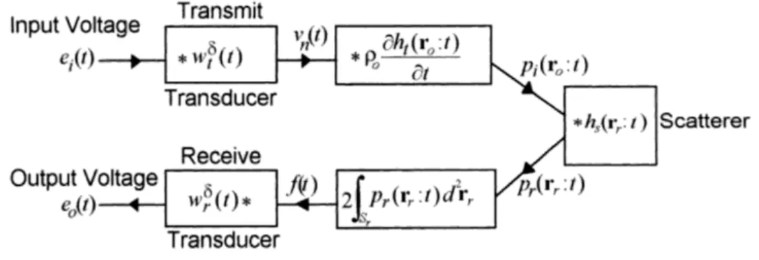
To describe the whole US image formation process (see Fig. 2.7), a setup given in Fig. 2.10 shall be considered. It is assumed that wave propagation is linear, non- attenuative, and non-dispersive, whereas variations in the acoustic properties of the medium should be small enough that only the incident wave is scattered (known as the Born approximation, see Section 2.2.5). Considering a single scatterer atr0, in order to obtain the output voltage the following equations can be formulated [37, p. 301] assuming a linear pulse-echo system (see Fig. 2.11):
pr(rr, t) =ei(t)∗wδt(t)∗ρ0∂ht(r0, t)
∂t ∗hs(rr, t) , (2.53) f(t) = 2
Z
Sr
pr(rr, t)d2rr, (2.54)
Figure 2.10: Geometry of a setup to determine the transmit-receive response of a system in the case of a single point scatterer. Picture taken from [37, p. 302].
Figure 2.11: The transmit and receive responses in the case of a single point scatterer, assuming a non-attenuating medium. Picture taken from [37, p. 302].
e0(t) =f(t)∗wrδ(t), (2.55) wherepr(rr, t) is the pressure distribution on the surface of the receiver transducer, ei(t) is the input voltage, wδt(t) and wδr(t) are the electromechanical responses of the transmit and receive transducers, respectively, ht(ro, t) is the velocity potential impulse response, hs(rr, t) is the pressure impulse response of the scatterer (the scattered pressure at an observation point caused by the incident wave), f(t) is the total force acting on the surface of the receiver transducer, Sr and St are the area of the receive and transmit transducers, respectively. Substituting Eqs. (2.53)
and (2.54) into Eq. (2.55) the output voltage is described as:
e0(t) = ρ0ei(t)∗wtδ(t)∗∂ht(r0, t)
∂t ∗
2 Z
Sr
hs(rr, t)d2rr
∗wrδ(t). (2.56) The impulse response of a point scatterer can be determined as follows:
hs(rr, t) =s(t)∗ δ(t− |rr−r0|/c0)
4π|rr−r0| , (2.57)
wheres(t) stands for the scatterer strength. As a consequence, the integral term in Eq. (2.56) can be be written as:
2 Z
Sr
hs(rr, t)d2rr =s(t)∗ Z
Sr
δ(t− |rr−r0|/c0)
2π|rr−r0| d2rr =s(t)∗ht(r0, t) ; (2.58) therefore, Eq. (2.56) can be expressed as:
e0(t) =ρ0∂ei(t)
∂t ∗wtδ(t)∗ht(r0, t)∗ht(r0, t)∗wδr(t)
| {z }
PSF
∗s(t)
|{z}
SF
, (2.59) which detailed form of the convolution-based image formation model was provided by Stepanishen [75], where the output voltage (which can be converted to pressure) can be calculated as the convolution between the point-spread function (PSF) of the system (which is the response of the imaging system to a point scatterer) and the SF.
2.2.7 Shift-invariant convolution model
The shift-invariant convolution model is a simplification of the shift-variant convolution model, which itself depends on several assumptions [34, 35] (see Sec- tion 2.2.6). Using such assumptions, it was shown that the RF image I can be estimated as the convolution of a SF with a PSF. Further assuming a spatially in- variant PSF, meaning that the position of the scatterer relative to the US transducer is irrelevant in the terms of impulse of the scattering, leads to the shift-invariant convolution model:
I = SF∗PSF, (2.60)
where ∗ is the spatially invariant convolution operator. According to the Fourier theorem, Eq. (2.60) can be rewritten in the Fourier domain as
F {I}=F {SF} F {P SF} , (2.61)
whereF {.} represents the 2-D Fourier transform operator.
In the current work the imaging model described above was used for simulating the US images in Chapter 3.
2.3 Theory of resolution enhancement
2.3.1 Mathematical formulation
As it has been discussed in Section 2.2.7, an US image can be described as the convolution of the SF with the PSF of the imaging system. In general, the degradation process can be written as a convolution with a PSF, along with some added noise (often considered as zero mean Gaussian white noise) as follows:
y[i, j] =
∞
X
k=−∞
∞
X
l=−∞
h[k, l]·x[i−k, j−l] +n[i, j], (2.62) wherey is the observed image, x is the SF (the underlying structure), h is the PSF of the imaging system (alternatively, transfer function), and n stands for the noise.
Equation (2.62) in a compact form reads as:
y=h∗x+n , (2.63)
where ∗ means the convolution operator. Equation (2.63) in the Fourier domain becomes:
Y =H.X+N , (2.64)
where the capital letters denote the Fourier transforms of Y, H, X and N, re- spectively, and . stands for the element-wise multiplication. Estimating X seems straightforward in the absence of noise if the PSF is known, as it becomes a simple multiplication with the inverse of the Fourier spectrum of the PSF H−1; however, there are many difficulties with this approach. From Eq. (2.64) it is obvious that separation of the H.X product leads to an ill-posed problem, as it is not guaran- teed that H−1 either exists or is unique, and noise also leads to inexact solutions.
Furthermore, even if H−1 exists but the matrix is not well-conditioned, then regu- larization needs to be performed beforehand in order to limit the effect of noise (ifH