The project was supported by the European Union, co-financed by the European Social Fund (EFOP-3.6.3-VEKOP-16-2017-00002).

(1)

A new angle on light-sheet microscopy and real-time image processing

Bálint Balázs

Pázmány Péter Catholic University Faculty of Information Technology and Bionics Roska Tamás Doctoral School of Sciences and Technology

Advisor: Balázs Rózsa, M.D., Ph.D.

A thesis submitted for the degree of Doctor of Philosophy

2018

(2)

Abstract

Light-sheet fluorescence microscopy, also called single plane illumination microscopy, has numerously proven its usefulness for long term imaging of embryonic development. This thesis tackles two challenges of light-sheet microscopy: high resolution isotropic imaging of delicate, light-sensitive samples, and real-time image processing and compression of light-sheet microscopy images.

A symmetric light-sheet microscope is presented, featuring two high numerical aperture objectives arranged in 120^◦. Both objectives are capable of illuminating the sample with a tilted light-sheet and detecting the fluorescence signal. This configuration allows for multi-view, isotropic imaging of delicate samples where rotation is not possible. The optical properties of the microscope are characterized, and its imaging capabilities are demonstrated on Drosophila melanogaster embryos and mouse zygotes.

To address the big data problem of light-sheet microscopy, a real-time, GPU-based image processing pipeline is presented. Alongside its capability of performing commonly required preprocessing tasks, such as image fusion of opposing views immediately during image acquisition, it also contains a novel, high-speed image compression method. This algorithm is suitable for both lossless and noise-dependent lossy image compression, the latter allowing for a significantly increased compression ratio, without affecting the results of any further analysis. A detailed performance analysis is presented of the different compression modes for various biological samples and imaging modalities.

(3)

List of Figures

1.1 Tradeoffs in fluorescence microscopy for live imaging . . . 4

1.2 Excitation and emission spectrum of enhanced green fluorescent protein (EGFP) . . . 4

1.3 Wide-field fluorescence microscope . . . 6

1.4 Axial cross section of the PSF and OTF of a wide-field microscope . . . . 8

1.5 Airy pattern . . . 9

1.6 Optical path length differences in the Gibson-Lanni PSF model . . . 11

1.7 Resolution of a wide-field microscope . . . 12

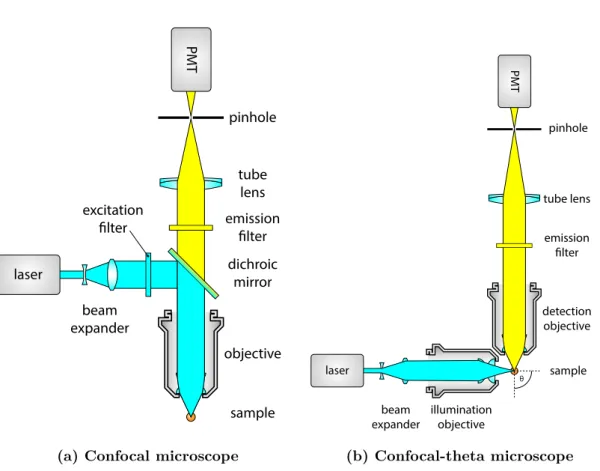
1.8 Basic optical components of a confocal laser scanning and confocal-theta microscope . . . 14

1.9 Axial cross section of the PSF and OTF of a confocal laser scanning microscope . . . 15

1.10 Basic concept of single-plane illumination microscopy . . . 16

1.11 Different optical arrangements for light-sheet microscopy . . . 17

1.12 Basic optical components of a SPIM . . . 19

1.13 Light-sheet dimensions . . . 21

1.14 DSLM illumination . . . 22

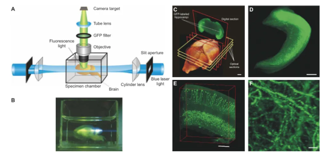
1.15 Inverted light-sheet microscope for multiple early mouse embryo imaging. 25 1.16 Imaging mouse post-implantation development . . . 26

1.17 Imaging adult mouse brain with light-sheet microscopy. . . 28

2.1 Dual view concept with high NA objectives . . . 31

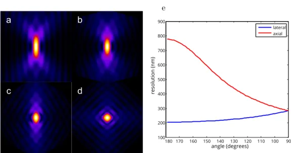
2.2 Lateral and axial resolution of a multi-view optical system . . . 33

2.3 Dual Mouse-SPIM optical layout . . . 35

2.4 The core unit of the microscope . . . 36

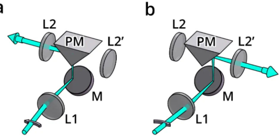
2.5 Illumination branch splitting unit . . . 38

2.6 Detection branch switching unit . . . 40

2.7 Microscope control hardware and software architecture . . . 45

2.8 Digital and analog control signals . . . 45

(6)

LIST OF FIGURES

2.9 Completed DualMouse-SPIM . . . 47

2.10 Stability measurements of view switcher unit . . . 49

2.11 Illumination beam profile . . . 50

2.12 Simulated and measured PSF of Dual Mouse-SPIM . . . 52

2.13 Combined PSF of 2 views . . . 52

2.14 Maximum intensity projection of a Drosophila melanogaster embryo recording . . . 54

2.15 Multi-view recording of a mouse zygote . . . 54

3.1 Building the binary Huffman tree . . . 61

3.2 Context for pixel prediction . . . 64

4.1 Experiment sizes and data rate of different imaging modalities . . . 67

4.2 Real-time image processing pipeline for multiview light-sheet microscopy . 67 4.3 Operating principle of MuVi-SPIM . . . 68

4.4 multiview fusion methods for light-sheet microscopy . . . 70

4.5 Classes of LVCUDA library . . . 71

4.6 Applying mask to remove background . . . 72

4.7 Comparison of 3D and 2D fusion of beads . . . 73

4.8 GPU fused images of a Drosophila melanogaster embryo . . . 75

4.9 Image contrast depending on z position for raw and fused stacks . . . 75

4.10 B³D algorithm schematics . . . 78

4.11 Options for noise-dependent lossy compression . . . 80

4.12 Theoretical and measured increase in image noise for WNL compression . 81 4.13 Compression performance . . . 84

4.14 Image quality of a WNL compressed dataset . . . 84

4.15 Compression error compared to image noise . . . 85

4.16 Influence of noise-dependent lossy compression on 3D nucleus segmentation 85 4.17 Influence of noise-dependent lossy compression on 3D membrane segmentation . . . 86

4.18 Influence of noise-dependent lossy compression on single-molecule localization . . . 86

4.19 Change in localization error only depends on selected quantization step . 87 C1 Light collection efficiency of an objective . . . 98

D1 3D model of DualMouse-SPIM . . . 100

(7)

List of Tables

3.1 Examples of a random binary code (#1) and a prefix-free binary code (#2) 59

3.2 Letters to be Huffman coded and their probabilities . . . 60

3.3 Huffman code table . . . 62

B1 Data sizes in microscopy . . . 96

B2 Lossless compression performance . . . 96

B3 Datasets used for benchmarking compression performance . . . 97

(8)

List of Abbreviations

2D two-dimensional.

3D three-dimensional.

BFP back focal plane.

CCD charge coupled device.

CLSM confocal laser scanning microscopy.

CMOS complementary metal oxide semiconductor.

CPU central processing unit.

DCT discrete cosine transform.

DFT discrete fourier transform.

DPCM differential pulse code modulation.

DSLM digitally scanned light-sheet microscopy.

dSTORM direct stochastic optical reconstruction microscopy.

DWT discrete wavelet transform.

eCSD electronic confocal slit detection.

EM-CCD electron multiplying CCD.

FEP fluorinated ethylene propylene.

FN field number.

FOV field of view.

FPGA field programmable gate array.

fps frames per second.

FWHM full width at half maximum.

GFP green fluorescent protein.

GPU graphics processing unit.

HEVC high efficiency video codec.

ICM inner cell mass.

(9)

List of Abbreviations

JPEG joint photographic experts group.

LSFM light-sheet fluorescence microscopy.

MIAM multi-imaging axis microscopy.

MuVi-SPIM Multiview SPIM.

NA numerical aperture.

OPFOS orthogonal plane fluorescent optical sectioning.

OTF optical transfer function.

PEEK polyether ether ketone.

PSF point spread function.

RESOLFT reversible saturable optical fluorescence transitions.

ROI region of interest.

sCMOS scientific CMOS.

SMLM single molecule localization microscopy.

SNR signal-to-noise ratio.

SPIM single-plane illumination microscopy.

STED stimulated emission depletion.

TE trophoectoderm.

TLSM thin light-sheet microscopy.

WNL within-noise-level.

YFP yellow fluorescent protein.

(10)

Introduction

Imaging techniques are one of the most extensively used tools in medical and biological research. The reason for this is simple: visualizing something invisible to the naked eye is an extremely powerful way to gain insight into its inner workings. Our brain has evolved to receive and process a multitude of signals from various sensors, and arguably the most powerful of these is vision.

As a branch of optics, microscopy (from ancient Greek mikros, “small” and skopein,

“to see”) is based on observing the interactions of light with an object of interest, such as a cell. To be able to see these interactions, the optics of the microscope magnifies the image of the sample, which can be recorded on a suitable device. For the first microscopes in the 17^th century, this was just an eye at the end of the ocular, and the recording was a drawing of the observed image [1].

Microscopy is a truly multidisciplinary field: even in its simplest form, just using a single lens, the principles of physics are applied to gain a deeper understanding of biology and nature. Today, microscopy encompasses most of natural sciences and builds on various technological advancements. While physics and biology are still in the main focus, the principles of chemistry (fluorescent molecules), engineering (automation) and computer science (image analysis) are all integrated in a modern microscopy environment.

Light-sheet fluorescence microscopy (LSFM), also called single-plane illumination microscopy (SPIM), is a relatively new addition to the arsenal of tools that comprise light microscopy methods, and is especially suitable for live imaging of biological samples, from within cells to entire embryos, over extended periods of time [2–5]. It is also eas- ily adapted to the sample, allowing to image a large variety of specimens, from entire organs [6], to the subcellular processes occurring inside cultured cells [7]. Due to its ability to bridge large scales in space and time, light-sheet microscopy can provide an unprecedented amount of information on biological processes. Despite its indubitable benefits, operating such a microscope can pose serious infrastructural challenges, as a single overnight experiment can generate tens of terabytes of data.

This work tackles two challenges in light-sheet microscopy: high-resolution live imaging of delicate samples, such as mouse embryos, and real-time image processing and compression of large light-sheet datasets. Before discussing the work in detail, Chapter 1

(11)

and Chapter 3 will give a short introduction to the concepts this thesis builds on. The basics of fluorescence microscopy, light-sheet microscopy, information theory and image compression will be covered.

Chapter 2 is devoted to presenting a new light-sheet microscope, the Dual Mouse- SPIM, designed for isotropic imaging of light-sensitive specimens. This microscope is based on two identical objectives positioned in 120^◦ as opposed to the conventional 90^◦ orientation used in light-sheet microscopy, and it offers dual-view detection through both lenses. We discuss the benefits of this arrangement and the design principles and optical layout of the microscope. After characterizing the optical properties of the microscope, we demonstrate its imaging capabilities on various samples.

In Chapter 4 we present a GPU-based real-time image processing pipeline designed to efficiently handle large amounts of microscopy data. As 3D imaging is gaining more and more traction, image datasets are generated at a faster pace than ever. We present a real-time preprocessing solution for multiview light-sheet microscopy, and a new image compression algorithm to significantly reduce data size by taking image noise into account. The theory behind these methods will be discussed before demonstrating their capabilities and evaluating their performance on multiple biological samples.

Finally, Chapter 5 will give a summary of the new results presented in this thesis, and discuss the potential future applications.

(12)

Chapter 1

Live imaging in three dimensions

Live imaging is indispensable to understand the processes at the interface of cell and developmental biology. In an ideal setting, the ultimate microscope would be able to record a continuos, three dimensional (3D), multicolor dataset of any biological process of interest with the highest possible resolution. Due to several limitations in physics and biology this is not possible. Therefore, a compromise is necessary. The diffractive nature of light, the lifetime of fluorescent probes and the photosensitivity of biological specimens all require microscopy to be adapted so that the question at hand may be answered.

In order to acquire useful data, one has to choose a tradeoff between spatial and temporal resolution and signal contrast, while making sure the biology is not affected by the imaging process itself [8]. This challenge can be illustrated by a pyramid where each corner represents one of these criteria (Figure 1.1), while a point inside the pyramid corresponds to the imaging conditions. As soon as we try to optimize one condition, i.e., we move the point closer to one of the corners, it will move further from all the others due to the limited photon budget. In order to make a fundamental difference and move the corners of the pyramid closer together, an change in microscope design is necessary.

1.1 Wide-field fluorescence microscopy

Fluorescence microscopy [9, 10], as a subset of light microscopy, is one of the few methods that allow subcellular imaging of live specimens with specific labeling. The first use of the term fluorescence is credited to George Gabriel Stokes [11], and it refers to the phenomenon of light emission following the absorption of light or other electromagnetic radiation. As the name fluorescence microscopy suggests, this method collects fluorescent light from the specimens. Since biological tissues are usually not fluorescent, except for some autofluorescence mostly at shorter wavelengths, fluorescent dyes or proteins have to be introduced to the system in order to be able to collect the necessary information.

The advantage of this is that the signal of the labeled structures will be of very high

(13)

1.1 Wide-field fluorescence microscopy

High Speed

High Contrast

Low Photodamage

High Resolution

Figure 1.1: Tradeoffs in fluorescence microscopy for live imaging. Also called the “pyramid of frustration”. When optimizing the imaging conditions (red dot), a tradeoff has to be made between resolution, contrast, and imaging speed, while avoiding photodamage. One can only be improved at the expense of the others due to the limited photon budget of the fluorescent molecules. Adapted from [8].

350 400 450 500 550 600 650

Wavelength (nm) 0

0.2 0.4 0.6 0.8 1 1.2

%T

Stokes shift

excitation emission

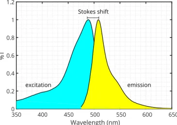
Figure 1.2: Excitation and emission spectrum of enhanced green fluorescent protein (EGFP).

Excitation spectrum in blue, emission spectrum in yellow. The separation between the two spectra is due to the Stokes shift, which is 19 nm for EGFP. Emission and excitation light can be separated by a long-pass filter at500 nm. Data from [12].

ratio compared to the background.

A fluorescent molecule is capable of absorbing photons in a given wavelength range (excitation spectrum) and temporarily store its energy by having an electron in a higher energy state, i.e., in an excited state. This excited state, however, is not stable, and the electron quickly returns to the ground state while emitting a photon. The energy of the absorbed and emitted photons are not the same, as energy loss occurs due to internal relaxation events, and the emitted photon has lower energy than the absorbed photon.

This phenomenon is called the Stokes shift, or red shift, and can be exploited in microscopy to drastically increase the signal-to-noise ratio by filtering out the illumination light (Figure 1.2).

(14)

1.1.1 Fluorescent proteins

Traditionally, synthetic fluorescent dyes were used to label certain structures in the specimens. Some of these directly bind to their target, and others can be used when conjugated to an antibody specific to the structure or protein of interest. A requirement for these methods is that the fluorescent label has to be added to the sample from an external source, and, in many cases, this also necessitates sample preparation techniques incompatible with live imaging, such as fixation [13].

The discovery of fluorescent proteins has revolutionized fluorescence microscopy.

Since these molecules are proteins, they can be produced directly by the organism if the proper genetic modifications are performed. Even though this was a hurdle at the time of discovering the green fluorescent protein (GFP) [14], genetic engineering techniques evolved since then [15], and not only has its gene been successfully integrated in the genome of a multitude of organisms [16–18], but many variants have been also engineered by introducing mutations to increase fluorescence intensity, and to change the fluorescence spectrum to allow multicolor imaging [18–21]. The usefulness and impact of these proteins are so profound, that in 2008 the Nobel Prize in chemistry was awarded to Osamu Shimomura, Martin Chalfie, and Roger Tsien “for the discovery and development of the green fluorescent protein, GFP” [22].

1.1.2 Wide-field image formation

By imaging fluorescently labelled specimens, a wide-field fluorescence microscope has the capability of discriminating illumination light from emitted fluorescent light due to the Stokes shift described in the previous section. The microscope’s operating principle is depicted in Figure 1.3.

Light from a source, typically a mercury lamp is focused on the back focal plane of the objective to create even illumination of the sample. Before entering the objective, the light is filtered, so only the wavelengths that correspond to the excitation properties of the observed fluorophores are transmitted. Since the same objective is used for both illumination and detection, a dichroic mirror is utilized to decouple the illumination and detection paths. The emitted light is filtered again to make sure any reflected and scattered light from the illumination source is blocked to increase signal-to-noise ratio.

Finally, light is focused by a tube lens to create a magnified image on the camera sensor.

This type of arrangement is called infinity-corrected optics, since the back focal point of the objective is in “infinity”, meaning that the light from a point source exiting the back aperture is parallel. This is achieved by placing the sample exactly at the focal point of the objective. Infinity-corrected optics have the advantage that they allow placing various additional optical elements in the infinity space, (i.e., the space between the objective and the tube lens) without affecting the image quality. In this example such elements

(15)

CAM

tube lens emission

ﬁlter light

source

excitation ﬁlter

dichroic mirror

objective

sample f α

r

Figure 1.3: Wide-field fluorescence microscope. The light source is focused on the back focal plane of the objective to provide an even illumination to the sample. Emitted photons are collected by the objective, and are separated from the illumination light by a dichroic mirror. Inset: Light collection of an objective lens.α: light collection half-angle;f: focal length;r: radius of aperture.

are the dichroic mirror and the emission filter.

The combination of the objective and tube lens together will determine the optical magnification of the system, which will be the ratio of the focal lengths of these lenses:

M = f_{T L}

f_OBJ. (1.1)

The final field of view (FOV) of the microscope will depend on the magnification, the size of the imaging sensor (D), and the objective field number (F N, specified by the manufacturer, the diameter of the view field in the image plane):

F OV = min(D, F N)

M . (1.2)

Apart from the magnification, the most important property of the objective is the half-angle of the light acceptance cone, α (Figure 1.3, inset). This not only determines the amount of collected light, but also the achievable resolution of the system (see Sec- tion 1.1.3). This angle depends on the size of the lens relative to its focal length. In other

(16)

words it depends on the aperture of the lens, which is why the expression numerical aperture (NA) is more commonly used to express this property of the objective:

NA =n·sinα, (1.3)

wherenis the refractive index of the medium, and describes the light propagation speed in the medium relative to the speed of light in vacuum. For vacuum and air n= 1, for watern_H₂_O= 1.33, and for the commonly used optical glass BK7n_BK7 = 1.52.

For smallα angles, the following approximation holds true:sinα≈tanα≈α. Thus, the numerical aperture can also be expressed as a ratio of the radius of the lens and the focal length:

NA≈nr

f, when α≪1. (1.4)

1.1.3 Resolution of a wide-field microscope

The resolution of an optical system depends on the size of the smallest distinguishable feature on the image. A practical way of quantifying this is by measuring the smallest resolved distance, i.e., the minimum distance between two point-like objects so that the two objects can still be distinguished. This mainly depends on two factors: the NA of the objective, and the pixel size of the imaging sensor.

Even if the imaging sensor would have infinitely fine resolution, it is not possible to reach arbitrarily high resolutions due to the wave nature of light and diffraction effects that occur at the aperture of the objective. This means that depending on the wavelength of the light, any point source will have a finite size on the image, it will be spread out, limiting the resolution. The shape of this image is called the point spread function, or PSF (Figure 1.4), as this function describes the behavior of the optical system when imaging a point-like source. This property of lenses was already discovered by Abbe in 1873 [23], when he constructed his famous formula:

δ= λ

2·NA. (1.5)

where δ is the smallest distance between two distinguishable features.

Another representation of the optical performance, is the optical transfer function, or OTF (Figure 1.4), which is the Fourier transform of the PSF:

OTF=F(PSF). (1.6)

As this function operates in the frequency space, it describes how the different spatial frequencies are affected by the system. The resolution can also be defined as the maximum of the support of the OTF, since this describes the highest frequency that is still

(17)

100 150 200 250

100

150

200

250

0 0.002 0.006 0.014 0.03 0.061 0.124 0.25 0.5 1

120 140 160 180 200

120 130 140 150 160 170 180 190

200 0

0.2 0.4 0.6 0.8 1

PSF OTF

Figure 1.4: Axial cross section of the PSF and OTF of a wide-field microscope. Simulated PSF (left) and OTF (right) for a wide-field microscope with a water immersion objective (n= 1.33).N A= 1.1, λ= 510 nm. Intensity has been normalized relative to the maximum, and is visualized with different colors (see colorbar). For better visualization, the logarithm of the intensity is displayed for the PSF.

transmitted by the optical system. Any pattern with higher frequency will be lost, thus lies beyond the resolution limit. For circularly symmetric PSFs, the OTF will have real values. However, if this is not the case, the Fourier transform also introduces complex components.

Abbe’s formula can be derived from the scalar theory of diffraction using a paraxial approximation (Fraunhofer diffraction, [24]). It is useful to define the following optical coordinates instead of the commonly used Cartesian coordinates x,y and z:

v = 2πnr

λ₀ sinα, u= 8πnz λ₀ sin²α

2 (1.7)

where r =√

x²+y² is the distance from the optical axis, and α is the light collection angle as shown on Figure 1.3. In this system the intensity of the electric field in the focus of a lens is [25]:

H(u, v) =C₀

∫ ₁

0

J₀(vρ)e⁻ⁱ¹²^·^uρ²ρdρ

2

, (1.8)

where C₀ is a normalization constant, ρ = r/max(r) is the normalized distance from the optical axis, and J0 is the zeroth-order Bessel function of the first kind. This is also called the Born-Wolf PSF model, named after the original authors [24].

To determine the lateral resolution of the system, let’s substituteu = 0as the axial optical coordinate, and evaluate Equation 1.8 which will give the intensity distribution in the focal plane:

H(0, v) =C₀

∫ ₁

0

J₀(vρ)ρdρ

2

= (

2J₁(v) v

)2

, (1.9)

(18)

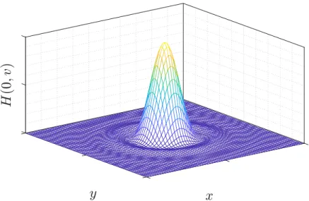
Figure 1.5: Airy pattern. Airy pattern calculated in Matlab based on Equation 1.9.

whereJ₁is the first-order Bessel function of the first kind. This equation describes the famous Airy pattern (Figure 1.5) which will be the shape of the PSF in the focal plane.

The width of this pattern will define the smallest resolvable distance, and although there are multiple definitions for this, the most commonly accepted is the Rayleigh criterion [24, 26]. It defines the resolution as the distance between the central peak and the first local minimum. As this lies at v= 3.38, the resolution can be expressed by substituting this value into Equation 1.7 and solving it for r:

δ_xy =r(v= 0.338) = 3.83 2π

λ₀

n·sinα ≈0.61 λ₀

N A, (1.10)

which is equivalent to Abbe’s original formula (Equation 1.5). The only difference is the scaling factor which is due to the slightly different interpretations of the width of the Airy disk as mentioned earlier.

Similarly, to calculate the intensity distribution along the axial direction, let’s sub- stitute v= 0 into Equation 1.8:

H(u,0) =C₀ (sin^u₄

u 4

)2

. (1.11)

For this expression the first minimum lies at u = 4π. Converting back to Cartesian coordinates, the axial resolution can be expressed as:

δ_z= 2nλ₀

N A². (1.12)

So far we only considered a single, point-like emitter. As the intensity function de-

(19)

scribes how an optical system “spreads out” the image of a point, it is also called the Point Spread Function (PSF, Figure 1.4). In a more realistic scenario, however the emit- ters are neither point-like, nor single. Effectively, however, for every emitter the PSF would be imaged on the sensor, and this creates the final image. In mathematical terms, this can be expressed as a convolution operation between the underlying fluorophore distribution of the object (O) and the PSF (H):

I(u, v) =O(u, v)∗H(u, v). (1.13) The effective result of this kind of diffraction-limited image formation is a blurred image with a finite resolution ofδ_xy in the lateral direction, andδ_z in the axial direction.

The PSF is further affected by the illumination pattern as well. Since the number of emitted fluorescent photons are roughly proportional to the illumination intensity, the illumination pattern will have an effect on the overall PSF of the system, which can be expressed as:

Hsys =Hill·Hdet, (1.14)

where H_ill is the point spread function of the illumination, andH_det is the point spread function of the detection.

1.1.4 Simulating the point spread function

To estimate the performance of a microscope, it is useful to simulate its point spread function. Usually this entails the numerical evaluation of the diffraction integral near the focal point. The most commonly used model for the PSF is the Born-Wolf model, which we already introduced in Equation 1.8. The only parameters for this model are the wavelength of the light (λ), the numerical aperture (NA), and the refractive index of the immersion medium (n). This model, however only accounts for an ideal image forming system without any aberrations.

For some experiments it is necessary to use the objectives in a slightly different environment than the original design conditions. Changes in the medium refractive index or coverslip thickness can lead to spherical aberrations, which are not accounted for in the Born-Wolf PSF model. The Gibson-Lanni model [27] gives a more general approach and it accounts for any differences between the experimental conditions and the design parameters of the objective, thus, it can simulate any possible aberrations that may arise.

The additional adjustable parameters are the thicknesses (t) and refractive indices (n) of the immersion medium (i), coverslip (g), and sample (s) (Figure 1.6).

Based of the parameters of the system,p = (NA,n,t), where n = (n_i, n^∗_i, n_g, n^∗_g, n_s) represents the refractive indices, and t = (ti, t^∗_i, tg, t^∗_g, ts) represents the medium thick-

(20)

optical axis

objective immersion

medium

ti coverslip

tg specimen

ts

ns ng ni

n^*_i n^*_i

P

Q

R

A

B C

D t^*_g t^*_i

S

designexperimental

zp O

z

Figure 1.6: Optical path length differences in the Gibson-Lanni PSF model. The optical path length difference is given by OP D = [ABCD]−[P QRS], where [ABCD] is the optical length of the experimental path (red), and[P QRS]is the optical length of the design path (blue). Adapted from [28].

nesses, the optical path difference can be calculated as:

OP D(ρ, z;z_p,p) = (z+t^∗_i)

√

n²_i −(NAρ)²+z_p√

n²_s−(NAρ)²−

−t^∗_i

√

(n^∗_i)²−(NAρ)²+t_g√

n²_g−(NAρ)²−t^∗_g√

(n^∗_g)²−(NAρ)²,

(1.15)

where ρ = r/max(r) is the normalized distance from the optical axis, z is the axial coordinate of the focal plane, and z_p is the axial location of the point source in the specimen layer. Then, the intensity near the focus can be expressed as:

H(u, v) =C

∫ ₁

0

J₀(vρ)e^iW^(ρ,z;z^p^,^p⁾ρdρ

2

, (1.16)

where the phase term W(ρ, z;z_p,p) = ^2π_λODP(ρ, z;z_p,p) and C is a constant complex amplitude.

Multiple software packages offer numerical evaluations of Equation 1.8 and Equa- tion 1.16. The ones extensively used in this thesis are the PSF Generator plugin [29] for Fiji [30], and MicroscPSF [28], which is implemented in Matlab. The PSF Generator supports the both PSF models, while MicroscPSF supports the Gibson-Lanni model. The latter implementation has the advantage that it is much faster due to the Bessel series approximation of the integral term, however, it only calculates the axial cross-section of the PSF. In contrast, PSF generator evaluates the integral for any specified 3D volume around the focal point.

(21)

1.2 Point scanning methods

0.0 0.2 0.4 0.6 0.8 1.0 1.2

0.11.010.0 051015202530axial

lateral axial/lateral

NA

Resolution (µm) axial/lateral ratio

Figure 1.7: Resolution of a wide-field microscope. Axial (blue) and lateral (red) resolutions of a wide-field microscope are shown with respect to the numerical aperture (NA). Resolutions are calculated withλ = 510nm, the emission maximum of GFP andn= 1.33, the refractive index of water, for water dipping objectives.

1.2 Point scanning methods

In most cases, a wide-field microscope is used to image a layer of cultured cells, or a sectioned sample, thus axial resolution is not a concern. Imaging live specimens, however is not so straightforward, as these samples are usually much thicker than a typical section.

For these samples 3-dimensional (3D) imaging is highly beneficial, which necessitates the use of optical sectioning instead of physical sectioning to be able to discriminate the features at different depths.

Due to the design of the wide-field microscope, any photons emitted from outside the focal plane will also be detected by the sensor, however as these are not originating from the focus, only a blur will be visible. This blur potentially degrades image quality and signal-to-noise ratio to such an extent that makes imaging thick samples very difficult if not impossible in a wide-field microscope.

Evaluating Equations 1.10 and 1.12 for a range of possible numerical apertures reveals the significant differences in lateral and axial resolution for any objective (Figure 1.7).

Especially for low NAs, this can be significant, a factor of ∼20 difference. For higher (>0.8) NAs the axial resolution increases faster than the lateral, however they will only be equal when α = 180^◦. This means that isotropic resolution with a single lens is only possible if the lens is collecting all light emitting from the sample, which seems hardly possible, and would be highly impractical. For commonly used high NA objectives the lateral to axial ratio will be around 3–6.

(22)

Instead of using a single lens to achieve isotropic resolution, it is more practical to image the sample from multiple directions to complement the missing information from different views. When rotating the sample by 90^◦ for example, the lateral direction of the second view will correspond to the axial direction of the first view. If rotation is not possible, using multiple objectives can also achieve similar results, such as in the case of Multi-Imaging Axis Microscopy (MIAM) [31, 32]. This microscope consisted of 4 identical objectives arranged in a tetrahedral fashion to collect as much light as possible from multiple directions, and provide isotropic 3D resolution, albeit at the expense of extremely difficult sample handling, since the sample was surrounded by objectives from all directions.

1.2.1 Confocal laser scanning microscopy

Confocal laser scanning microscopy (CLSM) [33, 34] addresses most of the problems of wide-field microscopy we mentioned in the previous section. It is capable of optical sectioning by rejecting out-of-focus light, which makes it a true 3D imaging technique.

Furthermore, the light rejection also massively reduces out-of-focus background, and increases contrast.

This is achieved by two significant modifications compared to the wide-field optical path. To be able to reject the out-of-focus light, an adjustable pinhole is placed at the focus of the tube lens. Light rays originating from the focal point will meet here, and are able to pass through the pinhole. However, out-of-focus light will converge either before or after the aperture, and thus the aperture blocks these rays. To maximize the fluorescence readout efficiency for the single focal point, a photomultiplier tube is used instead of an area sensor (Figure 1.8a).

As only a small focal volume is detected at a time, the illumination light is also focused here by coupling an expanded laser beam through the back aperture of the objective.

This not only increases illumination efficiency (since other, not detected points are not illuminated), but has the added benefit of increasing the resolution as well. This is due to the combined effect of illumination and detection PSFs as described in Equation 1.14 (Figure 1.9). For Gaussian-like PSFs, the final resolution (along a single direction) can be calculated in the following way:

1 δ²_sys = 1

δ²_ill + 1

δ_det² , (1.17)

where δ_ill and δ_det are the resolutions for the illumination and detection, respectively.

Since the same objective is used for both illumination and detection, and the difference

(23)

laser

PMT

pinhole

tube lens emission

ﬁlter excitation

ﬁlter

dichroic mirror beam

expander

objective

sample (a) Confocal microscope

laser

tube lens

emission ﬁlter

detection objective

sample

PMT

pinhole

θ

illumination objective beam

expander

(b) Confocal-theta microscope

Figure 1.8: Basic optical components of a confocal laser scanning and confocal-theta micro- scope. Both types of microscopes use confocal image detection, which means that a pinhole is used to exclude light coming from out-of-focus points. Light intensity is measured by a photomultiplier for every point in the region of interest. The final image is generated on a computer using the positions and recorded intensity values. A regular confocal microscope (a) uses the same objective for illumination and detection, while a confocal-theta microscope (b) uses a second objective that is rotated byθaround the focus. In this case,θ= 90^◦.

in wavelength is almost negligible, δ_ill=δ_det=δ, the final system resolution will be:

δ_sys= 1

√2δ. (1.18)

This means that the distinguishable features in a confocal microscope are ∼0.7 times smaller than in a wide-field microscope using the same objective.

Because of the different detection method in a confocal microscope, direct image formation on an area sensor is not possible, since at any given time only a single point is interrogated in the sample. Instead, it is necessary to move the illumination and detection point in synchrony (or in a simpler, albeit slower solution, to move the sample) to scan the entire field of view. The image can be later computationally reconstructed by a computer program that records the fluorescence intensity of every point in the field of view, and displays these values as a raster image.

(24)

100 150 200 250

100

150

200

250

0 0.002 0.006 0.014 0.03 0.061 0.124 0.25 0.5 1

120 140 160 180 200

120 130 140 150 160 170 180 190

200 0

0.2 0.4 0.6 0.8 1

PSF OTF

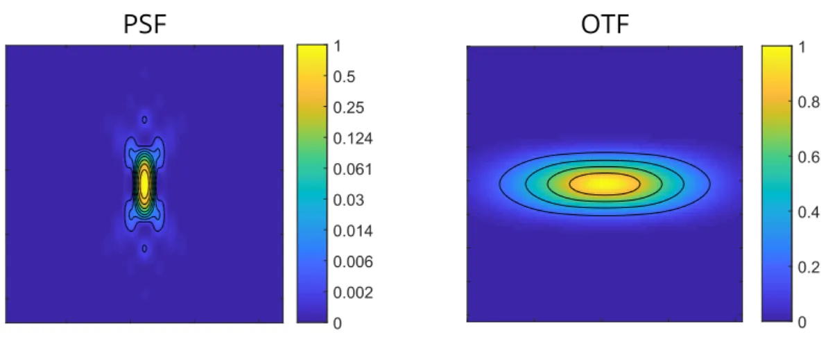
Figure 1.9: Axial cross section of the PSF and OTF of a confocal laser scanning microscope.

Simulated PSF and OTF for a laser scanning confocal microscope with a water immersion objective (n= 1.33). N A= 1.1,λ = 510 nm. Intensity has been normalized relative to the maximum, and is visualized with different colors (see colorbar). For better visualization, the logarithm of the intensity is displayed for the PSF.

1.2.2 Variants of confocal microscopy

Although confocal microscopy already has 3D capabilities, its axial resolution is still limited compared to the lateral, since it uses only one objective. An alternative realiza- tion of the confocal microscope, the confocal theta microscope [35] introduces a second objective to the system that is used to illuminate the sample (Figure 1.8b). Since this decouples the illumination and detection, using a dichroic mirror is no longer necessary.

The second objective is rotated by θ around the focus, this is where the name of this setup originates from.

As in the case of standard confocal microscopy, the system PSF is improved by the illumination pattern. Here, however, the axial direction of the detection coincides with the lateral direction of the illumination, which results in a dramatic improvement of axial resolution compared to standard confocal microscopy. Lateral resolution will also be increased, but by a smaller extent, resulting in an almost isotropic PSF and equal axial and lateral resolutions. Although this is a big improvement to confocal microscopy in terms of resolution, this technique did not reach a widespread adoption as it complicates sample handling, while still suffering from two drawbacks of confocal microscopy that limit its live imaging capabilities, namely phototoxicity and imaging speed.

One improvement to address these drawbacks is the use of a spinning disk with a specific pattern of holes (also called Nipkow disk) to generate multiple confocal spots at the same time [36]. If these spots are far enough from each other, confocal rejection of out-of-focus light can still occur. As the disk is spinning, the hole pattern will sweep the entire field of view, eventually covering all points [37]. The image is recorded by an area detector, such as a CCD or EM-CCD, which speeds up image acquisition [38].

(25)

1.3 Light-sheet microscopy

detection

specimen field of view

illumination

Figure 1.10: Basic concept of single-plane illumination microscopy. The sample is illuminated from the side by laser light shaped to a light-sheet (blue). This illuminates the focal plane of the detection lens, that collects light in a wide-field mode (yellow). The image is recorded, and the sample is translated through the light-sheet to acquire an entire 3D stack.

1.3 Light-sheet microscopy

A selective-plane illumination microscope (SPIM) uses a light-sheet to illuminate only a thin section of the sample (Figure 1.10). This illumination plane is perpendicular to the imaging axis of the detection objective and coincides with the focal plane. This way, only the section in focus will be illuminated, thus providing much better signal-to-noise ratio.

In case of conventional wide-field fluorescence microscopy, where the whole specimen is illuminated, out-of-focus light contributes to a significant background noise. With selective-plane illumination, this problem is intrinsically solved, and it also provides a true optical sectioning capability. This makes SPIM especially suitable for 3D imaging.

The main principle behind single-plane illumination microscopy, that is illuminating the sample from the side by a thin light-sheet, dates back to the early 20^thcentury, when Siedentopf and Zsigmondy first described the ultramicroscope [39]. This microscope used sunlight as an illumination source that was guided through a precision slit to generate a thin light-sheet. This allowed Zsigmondy to visualize gold nanoparticles floating in and out of the light-sheet by detecting the scattered light from the particles. Since these particles were much smaller than the wavelength of the light, the device was called an ultramicroscope. His studies with colloids and the development of the ultramicroscope led Zsigmondy to win the Nobel Prize in 1925.

After Zsigmondy this method was forgotten until rediscovered in the 1990s, when Voie et al. constructed their Orthogonal-plane Fluorescent Optical Sectioning (OPFOS) microscope [40]. They used it to image a fixed, optically cleared and fluorescently labelled guinea pig cochlea. In order to acquire a 3D dataset, the sample was illuminated from the side with a light-sheet generated by a cylindrical lens, then rotated around the center axis

(26)

a b c d

g f

e

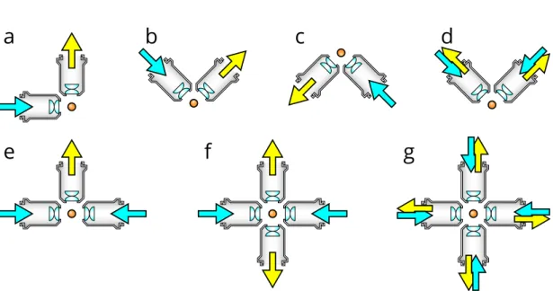
Figure 1.11: Different optical arrangements for light-sheet microscopy. (a) Original SPIM design with a single lens for detection and illumination. [43] (b) Upright SPIM to allow for easier sample mounting such as using a petri dish (iSPIM [44, 45, J1]). (c) Inverted SPIM, where the objectives are below the sample, which is held by a thin foil [J2]. (d) Dual-view version of the upright configuration, where both objective can be used for illumination and detection (diSPIM [46]). (e) Multidirectional-SPIM (mSPIM) for even illumination of the sample with two objectives for illumination [47]. (f) Multi-view SPIM with two illumination and detection objectives for in toto imaging of whole embryos (MuVi-SPIM [48], SimView [49], Four-lens SPIM [50]). (g) A combination of (d) and (f), using four identical objectives, where both can illuminate and detect in a sequential manner, to achieve isotropic resolution without sample rotation (IsoView [51]).

to obtain multiple views. Although they only reached a lateral resolution of around10µm and axial resolution of26µm, this method allowed them to generate a 3D reconstruction of the guinea pig cochlea [41].

Later, in 2002, Fuchs et al. developed Thin Light-Sheet Microscopy (TLSM) [42]

and used this technique to investigate the microbial life in seawater samples without disturbing their natural environment (by, e.g., placing them on a coverslip). Their light- sheet was similar to the one utilized in OPFOS, being 23µm thin, and providing a 1 mm×1 mmfield of view.

Despite these early efforts, the method did not gain larger momentum. The real breakthrough in light-sheet imaging happened at the European Molecular Biology Labo- ratory (EMBL) in 2004, where Huisken et al. [43] combined the advantages of endogenous fluorescent proteins and the optical sectioning capability of light-sheet illumination to image Medaka fish embryos, and the complete embryonic development of a Drosopila melanogaster embryo. They called this Selective-Plane Illumination Microscopy (SPIM), and it quickly became popular to investigate developmental biological questions.

Since then, light-sheet-based imaging has gained more and more popularity, as it can be adapted and applied to a wide variety of problems. Although sample mounting can be challenging because of the objective arrangement, this can also be an advantage, since

(27)

new microscopes can be designed with the sample in mind [3, J3] (Figure 1.11). This made it possible to adapt the technique for numerous other specimens, such as zebrafish larvae [52], C. elegans embryos [45], mouse brain [6], and even mouse embryos [J2, 53, 54].

As many of these specimens require very different conditions and mounting techniques, these microscopes have been adapted to best accommodate them. An upright objective arrangement (Figure 1.11b), for example, allows imaging samples on a coverslip, while its inverted version is well suited for mouse embryos, where a foil is separating the samples from the immersion medium (Figure 1.11c). A modified version of the upright arrangement allows for multi-view imaging using both objectives for illumination and detection in a sequential manner (Figure 1.11d) [55].

To achieve a more even illumination in larger samples, two objectives can be used from opposing directions to generate two light-sheets (Figure 1.11e) [47]. This arrangement can further be complemented by a second detection objective, to achieve parallelized multi-view imaging (Figure 1.11f) [48–50]. For ultimate speed, 4 identical objectives can be used to achieve almost instantaneous views from 4 different directions by using all objectives for illumination and detection (Figure 1.11g) [51].

Furthermore, because of the wide-field detection scheme it is possible to combine SPIM with many superresolution techniques, such as single molecule localization [56], STED [57], RESOLFT [J1], or structured illumination [7, 58, 59].

Since illumination and detection for light-sheet microscopy are decoupled, two independent optical paths are implemented.

The detection unit of a SPIM is largely equivalent to a detection unit of a wide-field microscope without the dichroic mirror (Figure 1.12). The most important components are the objective together with the tube lens, filter wheel, and a sensor, typically a charge coupled device (CCD) or scientific complementary metal–oxide–semiconductor (sCMOS) camera.

The resolution of a light-sheet microscope mainly depends on the detection objective.

Since imaging biological specimens usually requires a water-based solution, the objectives also need to be directly submerged in the medium to minimize spherical aberrations. As the refraction index of water (n= 1.33) is greater than the refraction index of air, these objectives tend to have a higher NA, resulting in higher resolution. As the illumination is decoupled in this system, the light-sheet thickness also has an influence on the axial resolution. Finally, the resolution also depends on the pixel size of the sensor which determines the spatial sampling rate of the image.

Although image quality and resolution greatly depend on the detection optics, the real strength of light-sheet microscopy is the inherent optical sectioning which is due to the specially aligned illumination pattern that confines light to the vicinity of the

(28)

CAM

laser

90°

tube lens

emission ﬁlter

detection objective

sample

light-sheet

illumination objective cylindrical

lens beam

expander

Figure 1.12: Basic optical components of a SPIM. A dedicated illumination objective is used to generate the light-sheet, which is an astigmatic Gaussian beam, focused along one direction. Astigmatism is introduced by placing a cylindrical lens focusing on the back focal plane of the objective. Detection is performed at a right angle, with a second, detection objective. Scattered laser light is filtered out, and a tube lens forms the image on an area sensor, such as an sCMOS camera.

detection focal plane.

There are two most commonly used options to generate a light-sheet: either by using a cylindrical lens to illuminate the whole field of view with a static light-sheet, as in the original SPIM concept [43]; or by quickly scanning a thin laser beam through the focal plane, thus resulting in a virtual light-sheet. This method is called Digitally Scanned Light-sheet Microscopy (DSLM) [52].

1.3.1 Static light-sheet illumination

For a static light-sheet, the normally circular Gaussian laser beam needs to be shaped in an astigmatic manner, i.e., either expanded or squeezed along one direction, to shape it into a sheet instead of a beam. This effect can be achieved by using a cylindrical lens,

(29)

which, as the name suggests, has a curvature in one direction, but is flat in the other, thus focusing a circular beam to a sheet (Figure 1.12).

However, to achieve light-sheets that are sufficiently thin for optical sectioning, one would need to use a cylindrical lens with a very short focal length, and these are hardly accessible in well corrected formats. For this reason, it is more common to use a longer focal length cylindrical lens in conjunction with a microscope objective, which is well corrected for chromatic and spherical aberrations [60]. This way, the light-sheet length, thickness and width can be adjusted for the specific imaging tasks.

Light-sheet dimensions

The shape of the illumination light determines the optical sectioning capability and the field of view of the microscope, so it is important to be able to quantify these measures.

The most commonly used illumination source is a laser beam coupled to a single mode fiber, thus its properties can be described by Gaussian beam optics.

For paraxial waves, i.e., waves with nearly parallel wavefront normals, the general wave equation can be approximated with the paraxial Helmholtz equation [61]

∇²TU+i2k∂U

∂z = 0, (1.19)

where ∇²T = _∂x^∂²2 +_∂y^∂²2,U(⃗r) is the wave function,k= ^2π_λ is the wavenumber andz is in the direction of the light propagation.

A simple solution to this differential equation is the Gaussian beam:

U(r, z) =A₀· W₀ W(z) ·e⁻

r2

W2(z) ·e^{−i·φ(r,z)}, (1.20) whereA₀ is the amplitude of the wave,W₀ is the radius of the beam waist (the thinnest location on the beam), r=√

x²+y² is the distance from the center of the beam, W(z) is the radius of the beam at distance zfrom the waist, andϕ(r, z)is the combined phase part of the wave-function. Furthermore:

W(z) =W₀

√ 1 +

( z z_R

)2

(1.21) where the parameter z_R is called the Rayleigh-range, and is defined the following way:

z_R = πW₀²

λ . (1.22)

Apart from the circular Gaussian beam, the elliptical Gaussian beam is also an eigen- function of Helmholtz equation (Equation 1.19) which describes the beam shape after a

(30)

2·W(z) 2·zR

w_fov h_fov

h_LS

(a)

−2 −1 0 1 2

0.00.51.01.52.0

z/zR

W0 √2·W0

2·zR

W/W0

(b)

−2 −1 0 1 2

0.00.20.40.60.81.0

2·z_R

normalized intensity

(c)

Figure 1.13: Light-sheet dimensions. (a) The light-sheet, with the field of view indicated. Since the light-sheet intensity is uneven, the field of view has to be confined to a smaller region. (b) The width and thickness of the field of view depends on the Rayleigh length of the beam (zR,y) and the beam waist (W0).

(c) The height of the field of view is determined by the Gaussian profile of the astigmatic beam.

cylindrical lens:

U(x, y, z) =A₀·

√ W_0,x W_x(z−z_0,x)

√ W_0,y

W_y(z−z_0,y)·e⁻

x2 W2

x(z−z0,x) ·e⁻

y2 W2

y(z−z0,y) ·e−i·φ(x,y,z). (1.23) This beam still has a Gaussian profile along the x and y axes, but the radii (W0,x and W_0,y), and the beam waist positions (z0,x and z_0,y) are uncoupled, which results in an elliptical and astigmatic beam. The beam width can now be described by two independent equations for the two orthogonal directions:

W_x(z) =W_0,x

√ 1 +

( z zR,x

)2

and W_y(z) =W_0,y

√ 1 +

( z zR,y

)2

. (1.24)

Since the beam waist is different along the two axes, the Rayleigh range is also different:

zR,x= πW_x,0²

λ , and zR,y = πW_y,0²

λ . (1.25)

Based on these equations, the light-sheet dimensions and usable field of view can be specified (Figure 1.13a). The light-sheet thickness will depend on the beam waist, W_0,y (if we assume the cylindrical lens is focusing along y), and the length of the light-sheet can be defined as twice the Rayleigh range, 2·z_R,y (Figure 1.13b). As these are coupled (see Equation 1.25), having a thin light-sheet for better sectioning also means that its length will be relatively short. Fortunately, because of the quadratic relation, to increase the field of view by a factor of two, the light-sheet thickness only needs to increase by a factor of √

2.

Light-sheet height is determined by the intensity profile of the beam along the vertical

(31)

CAM

90°

laser

tube lens

emission ﬁlter

detection objective

sample

virtual light-sheet

illumination objective tube

lens scan

lens scanning

mirror

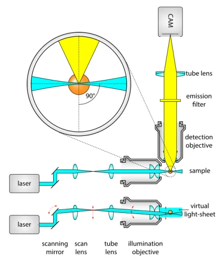
Figure 1.14: DSLM illumination. DSLM illuminates a specimen by a circularly-symmetric beam that is scanned over the field of view. This creates a virtual light-sheet, which illuminates a section of a specimen just like the SPIM. The light-sheet in DSLM is uniform over the whole field of view and its height can be dynamically altered by changing the beam scan range.

axis (Figure 1.13c). Since this is a Gaussian function (see Equation 1.20), only a small part in the middle can be used for imaging, because towards the sides the intensity dramatically drops. When allowing a maximum 20% drop-off in intensity at the edges, the light-sheet height becomes h_{f ov} = 2·0.472·Wx,0 = 0.944·Wx,0.

1.3.2 Digitally scanned light-sheet illumination

Although generating a static light-sheet is relatively straightforward with the simple addition of a cylindrical lens to the light path, it has some drawbacks. As already mentioned in the previous section, the light intensity distribution along the field of view is not constant, as the light-sheet is shaped from a Gaussian beam. Furthermore, along the lateral direction of the light-sheet the illumination NA is extremely low, resulting in effectively collimated light. Because of this, shadowing artifacts can deteriorate the image quality [47].

(32)

1.4 Light-sheet imaging of mammalian development

A more flexible way of creating a light-sheet is by scanning a focused beam in the focal plane to generate a virtual light-sheet (digital scanned light-sheet microscopy, DSLM [52]). Although this method might require higher peak intensities, it solves both drawbacks of the cylindrical lens illumination. By scanning the beam, the light-sheet height can be freely chosen, and a homogenous illumination will be provided. Focusing the beam in all directions evenly introduces more angles in the lateral direction as well, which shortens the length of the shadows.

The basic optical layout of a DSLM is shown on Figure 1.14. A galvanometer con- trolled mirror that can quickly turn around its axis is used to alter the beam path, which will result in an angular sweep of the laser beam. To change the angular movement to translation, a scan lens is used to generate an intermediate scanning plane. This plane is then imaged to the specimen by the tube lens and the illumination objective, resulting in a scanned focused beam at the detection focal plane. The detection unit is identical to the wide-field detection scheme, similarly to the static light-sheet illumination. By scanning the beam at a high frequency, a virtual light-sheet is generated, and the fluorescence signal is captured by a single exposure on the camera, resulting in an evenly illuminated field of view.

1.4 Light-sheet imaging of mammalian development

Live imaging of mammalian embryos is an especially challenging task due to the in- trauterine nature of their development. As the embryos are not accessible in their natural environment, it is necessary to replicate the conditions as closely as possible by providing an appropriate medium, temperature, and atmospheric composition. Moreover, these embryos are extremely sensitive to light, which poses a further challenge for microscopy [62]. lllumination with high laser power for an extended time frame can result in bleaching of the fluorophores, which in turn will lower the signal at later times. Furthermore, any absorbed photon has the possibility to modify the chemical bonds inside the specimen, which can lead to phototoxic effects, disrupting the proper development of the embryo.

Because of its optical sectioning capabilities combined with the high specificity of fluorescent labels, confocal microscopy has had an immense influence on biological research, and has been the go-to technique for decades for many discoveries [36, 63, 64]. Imaging live specimens for an extended period of time with confocal microscopy, although possible [65, 66], is not ideal. Due to the use of a single objective, for each voxel imaged, a large portion of the specimen has to be illuminated below and above the focal plane as well. This results in a high dose of radiation on the sample that can be as much as 30–100 times larger than the dose used for the actual imaging [67], depending on the number of planes recorded. Moreover, the usage of the pinhole, although rejects out-of-focus light,