DOI: 10.1556/606.2019.14.3.8 Vol. 14, No. 3, pp. 75–85 (2019) www.akademiai.com
NON-INTRUSIVE BEDLOAD GRANULOMETRY USING AUTOMATED IMAGE ANALYSIS
1 Daniel BUČEK*, 2 Martin ORFÁNUS, 3 Peter DUŠIČKA
1,2,3
Department of Hydraulic Engineering, Faculty of Civil Engineering Slovak University of Technology, Radlinského 11, 810 05, Bratislava, Slovakia e-mail: 1daniel.bucek@stuba.sk, 2martin.orfanus@stuba.sk, 3peter.dusicka@stuba.sk
Received 31 December 2018; accepted 21 May 2019
Abstract: This paper presents a proprietary open source code for analysis of granulometric properties of bed load material based on non-intrusive automated image analysis. Vertical bed- surface images are processed using the proposed tool and verified with results obtained by well tested optical granulometry tool Basegrain. The practical application of the proposed tool yields accuracy comparable that of the tested framework and traditional sampling methods.
Additionally, results showed that the average D50 grain-size sampled from riverbed of studied river section of river Danube agrees up to 95% with the average D50 sampled from riverbanks.
Keywords: Optical granulometry, Automated image analysis, Sediment transport, Open source
1. Introduction
Numerical morpho-dynamic models have been developed in the past 35 years and are widely applied by the engineering community to predict riverbed evolution. High processing power of currently available processors together with efficient numerical methods brought morpho-dynamic modeling to a state, where it can be used as a viable and powerful engineering tool even for large scale problems. Morpho-dynamic models are generally seen as much less accurate as hydrodynamic models. Main reason is the accumulation of errors, which are difficult to quantify [1]. Large amount of input data, which are difficult to measure in-situ is required to accurately describe sediment
* Corresponding Author
transport processes. Morpho-dynamic models are based on empirical sediment transport equations, which are derived from small scale experiments and their up-scaling for practical application in the field is questionable [2], [3]. With the aid of advanced first- order second-moment uncertainty method with algorithmic differentiation and Monte Carlo simulation, it was found that median grain-size D50 was found to contribute to up to 25% of variability in the morpho-dynamic model results. The other input parameters (empirical Meyer-Peter-Müller factor, bed roughness) are found to have secondary importance in the present application [4], [5].
The spatial variability of grain-size at a variety of scales makes the characterization of fluvial sediment problematic. Large sample sizes are necessary to ensure satisfactory representation of grain-size distribution and sampling is therefore time consuming and expensive. Conventional sampling techniques leave potentially important textural variations unresolved [6].
Development of more effective approaches to sampling that achieve satisfactory characterization of grain-size whilst reducing the time for analysis is highly desirable.
First attempts in optical grain analysis made use of film-based photography, but subsequent, manual analysis of the photographs was time-consuming if not impractical.
More advanced approaches to photo-sieving enable automated grain site analysis but still depend on manual identification of individual particles [7], [8]. Latest and probably the most advanced, freely distributable tool for optical granulometry Basegrain requires little to no user intervention and yields very high accuracy. It is distributed over the Internet in binary form (the source code remains closed). Any kind of code adaptation for specific use is currently not possible. Basegrain lacks process automation; therefore, its use is restricted to projects where handling and analyzing each sample image separately is feasible [9].
2. Material and methods
The aim of this paper is to introduce a non-intrusive grain-size analysis tool based on automated image analysis that is portable, open-source and enables process automation. It is compared to existing and well tested grain-size analysis tool Basegrain [9]. Both results are then compared to reference data gathered with traditional methods on river Danube in 1959, 1997 and 2003 [10]. Efforts to develop this tool arose from the need to densify a sparse dataset of grain-size distributions on river Danube in Slovakia, which is subject of another project with focus on morpho-dynamic modeling. Due to high costs of traditional sampling methods, the last available historical information on grain-size distribution is often used as an input variable for morpho-dynamic modeling.
The grain-size analysis tool presented consists of two separate scripts. First is an ImageJ macro for particle analysis from an image sample. The virtual photo sieving and plotting of results is handled by the second script written in Python programming language. The tool is written in a way to enable batch processing of large number of samples automatically in series, which crucially increases the efficiency of workflow.
The procedure of automated grain-size analysis is divided into four stages: sample image collection; image pre-processing; image processing and analysis; the derivation of a grain-size distribution.
Sample image collection. Input data for the procedure is an image of a patch of sediment collected roughly vertically with a digital camera. The scale of the image is such that the smallest grain of interest has a b-axis (the minor axis in the imagery) larger than 23 pixels. Experience indicated so far, that grains areas < ~20 px are hardly detected at all, as confirmed by Graham et al. [6], who found the limit of 23 px [6]. It is crucial, that sample images are taken in natural shadow, before dawn, right after dusk or during overcast to avoid any direct sunlight causing prominent directional shadow.
Patch of sampled sediment should be dry. Directional shadows together with reflections off of glossy wet surface optically distort the boundaries between individual grains thus introducing an error into the optical analysis result. Samples are collected at riverbanks, ideally at low water stage when they are sufficiently exposed. Since access to riverbanks from land is often complicated if not impossible, man-powered boat was used to travel downstream and collect sample images along the way. The advantage of this approach is easy deployment in various environments, carry ability and relatively low acquisition cost in comparison to other means of waterborne transportation e.g. motorboat.
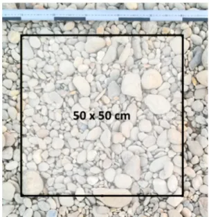
Image pre-processing. Sample image is manually cropped to square with side dimension of desired size, taking the measuring rod placed on the side of captured area as reference (Fig. 1). Radial distortion and perspective effect are not taken into consideration. Correction thereof showed to cause statistically insignificant change in final grain-size analysis results, unless the sample photos were taken at an obvious angle.
Fig. 1. Cropping the sample image to square of desired size (Source: Author)
Image processing and analysis. Color information is not required, so the first step is to convert the image to grayscale. The image is then manipulated by the application of a median filter, which smoothest markings on the grain surfaces but preserves edges.
Median filter reduces noise in the image by replacing each pixel with the median of the neighboring pixel values [11]. Optimal radius for median filter was in case of studied samples found to be 1.5 mm. First segmentation is obtained by a binary image of the gray-scale photograph with an Otsu’s thresholding method [12]. Otsu’s threshold clustering algorithm searches for the threshold that minimizes the intra-class variance, defined as a weighted sum of variances of the two classes [12]. This segmentation is then refined by watershed segmentation of the Euclidian Distance Map (EDM).
Watershed segmentation based on the EDM splits a particle if the EDM has more than one maximum (if there are several largest inscribed circles at different positions). This step requires the Adjustable Watershed ImageJ plugin, which enables to set tolerance of particle segmentation. This value determines the difference of radius between the smaller of the largest inscribed circles and a circle inscribed at the neck between the particles [13].
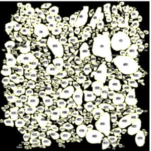
To analyze segmented particles, the algorithm Analyze particles are used. It works by scanning the image until it finds the edge of an object. It then outlines the object, measures it, fills it to make it invisible, then resumes scanning until it reaches the end of the image or selection [14]. The segmented images should be checked at this stage in case the segmentation has failed for some reason (Fig. 2). If necessary, watershed algorithm tolerance should be adjusted for optimal outcome. Optimal tolerance for this study was found to be at value 2.
Fig. 2. Segmented and detected particles (Source: Author)
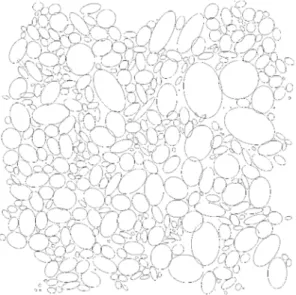
The selected objects are measured during the last step using an ellipse-fitting procedure to obtain the minor axis (Fig. 3). Approximating the b- or intermediate axis in conventional granulometry gives an unbiased estimate of the minor-axis length [6].
Results of the particle analysis are stored in comma delimited data file containing length of minor and major ellipse axis and area of segmented particles. Complete image
processing and particle analysis macro, which was developed during this study, was written in verbal form, so it is easy to follow (Code 1). The code includes simple data structure management to allow storage of the intermediary results, allowing the user to check for the quality of particle segmentation and particle detection.
Fig. 3. Ellipses fitted to particles (Source: Author)
Code 1. Image processing and particle analysis macro script for ImageJ (Source: Author)
#@File(label = "Input directory", style = "directory") input_Folder
#@Integer(label = "Width of square sample image (mm)") width_mm
#@Float(label = "Median filter radius (mm)") radius_mm
#@Float(label = "Watershed tolerance") tolerance
dir_in = input_Folder+File.separator;
dir_out = dir_in+".."+File.separator+"Output"+File.separator;
File.makeDirectory(dir_out);
list = getFileList(dir_in);
path_results = dir_out + "Results"+File.separator;
path_ellipses = dir_out + "Ellipses"+File.separator;
path_particles = dir_out + "Particles"+File.separator;
File.makeDirectory(path_results);
File.makeDirectory(path_ellipses);
File.makeDirectory(path_particles);
setBatchMode(true);
for (i=0; i<list.length; i++) {
path = dir_in+list[i];
open(path);
run("Clear Results");
width_px = getWidth();
radius_px = radius_mm/width_mm*width_px;
run("Median...", "radius=radius_px");
run("8-bit");
setAutoThreshold("Otsu dark");
run("Convert to Mask");
run("Adjustable Watershed", "tolerance=tolerance");
run("Set Measurements...", "area fit display add redirect=None decimal=3");
run("Set Scale...", "distance=width_px known=width_mm pixel=1 unit=mm");
run("Analyze Particles...", " show=Ellipses exclude clear include add");
name = File.nameWithoutExtension;
saveAs(".png", path_ellipses + name +
"_Ellipses_r="+radius_mm+"mm_"+"tolerance="+tolerance+".png");
close();
saveAs("Results", path_results + name +
"_Results_r="+radius_mm+"mm_"+"tolerance="+tolerance+".csv");
run("Revert");
setMinAndMax(130, 250);
run("Flatten");
saveAs(".png", path_particles + name +
"_Particles_r="+radius_mm+"mm_"+"tolerance="+tolerance+".png");
close("*");
}
Derivation of a grain-size distribution. Graham et al. [6] suggests that use of a single average flatness index is unlikely to introduce a significant bias to the grain-size distributions for most lithologies. It should be necessary to survey the flatness index only if the sediment is characterized by exceptionally flat or spherical grains, otherwise it is recommended to use a sieve-correction factor of 0.79 (corresponding to a flatness index of 0.51) [6]. The sieve-corrected b-axes measurements may be used directly to generate a cumulative grain-size distribution.
For this purpose, a function in Python programming language was written, which reads the result data file and returns cumulative grain-size distribution together with median grain-size D50. The function is divided into four steps.
• First step applies sieve-correction factor of 0.79 to the b axis (or minor axis) of each grain [6];
• Second step contains the virtual sieving algorithm, which compares each grains b-axis with iteratively increasing size of sieve opening and calculates the percentage of particles, which pass through the sieve. The sieve size increases at 1 mm increments from 0 mm up to the b axis of largest particle;
• Third step serves to obtain D50 grain-size by fitting the data with fifth degree polynomial and calculating the only root for 50% of its inverse cumulative distribution function that belongs to the interval between 0 mm and largest grain-size;
• The final step manages comprehensive plotting of the grain-size analysis. Plot of cumulative grain-size distribution is saved in the Output directory together with calculated D50 grain-size. Complete content of the script for calculating the grain-size distribution and D50 is written in verbal form to be easy to follow (Code 2).
Code 2. Algorithm for calculating the grain-size distribution and D50 grain-size written in Python (Source: Author)
from os import listdir from os.path import isfile, join import pandas as pd
import numpy as np
import matplotlib.pyplot as plt
def sieve_analysis(results_dir):
result_files = [f for f in listdir(results_dir) if isfile(join(results_dir, f))]
result_files = [f for f in result_files if '.csv' in f]
for j in result_files:
data = pd.read_csv(results_dir+'/'+j) area = data['Area']
num_of_particles = len(data) total_area = area.sum()
# sieve-correction factor of 0.79 (corresponding to a flatness index of 0.51) minor_axis = (data['Minor'])*0.79
largest_grain = round(minor_axis.max()+0.5) # sieving algorithm
sieve = np.arange(0,largest_grain,1) cummulative_sum = []
area_passing_percentage = []
for opening in sieve:
area_passing = (area.where(minor_axis<opening).sum()) cummulative_sum.append(area_passing)
area_passing_percentage.append(area_passing/total_area*100) # calculate D50, D90
Di = {}
for i in [50, 90]:
best_fit = np.polyfit(sieve, area_passing_percentage, 5) p = np.poly1d(best_fit)
roots = (p - i).roots
n = [n for n in roots if (np.isreal(n) and n > 0 and n < largest_grain)]
Di.update({'D'+str(i) : str((round(float(np.real(n)), 1)))}) # plot
file_name = j.strip('.csv').split('_')
label = file_name[0]+' '+file_name[1]+' D50 = '+str(Di['D50'])+' mm '+'D90 = '+str(Di['D90'])+' mm ('+str(num_of_particles)+' particles, w.s. tolerance = '+file_name[- 1].strip('tol=')+')'
plt.plot(sieve, area_passing_percentage, label=label) plt.legend(fontsize=7, loc=4)
plt.xlabel('Di (mm)')
plt.ylabel('Larger than Di (%)') plt.title('Sieve Analysis ')
plt.xticks(np.arange(0,largest_grain,5)) plt.yticks(np.arange(0,110,10))
plt.grid(which='major', linestyle='--', color='grey')
plt.savefig(results_dir+'/../'+'Sieve_Analysis.png',bbox_inches='tight', dpi=300) plt.close('all')
3. Results and discussion
Sample images were taken on river Danube at km 1865, km 1872 and km 1876.
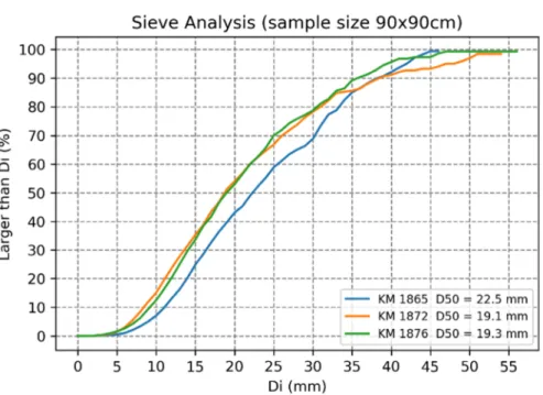
Images were cropped to size 50x50 cm and 90x90 cm for comparison. Granulometric analysis was performed by proposed tool and compared against results obtained by optical granulometry tool Basegrain. Cumulative grain-size distribution derived from sample images with size 90x90 cm is significantly smoother than that of 50x50 cm yet the overall change of D50 value does not exceed 5%. Average absolute deviation between results obtained by Basegrain and proposed tool is 5.2% for sample size 50x50 cm and 5.6% for sample size 90x90 cm. Individual absolute deviation does not exceed 10% (Fig. 4, Fig. 5, Table I, Table II).
Fig. 4. Cumulative grain-size distribution derived from sample image of size 50x50cm (Source: Author)
Fig. 5. Cumulative grain-size distribution derived from sample image of size 90x90cm (source: Author)
Table I
D50 obtained by proposed tool compared against D50 obtained by Basegrain
River km
Sample size 50x50 cm Proposed
tool (mm)
BASEGRAIN (mm)
Deviation (%)
Average deviation
(%)
1876 20.4 21.4 4.7
5.2
1872 19.8 22.0 10.0
1865 21.9 21.7 0.9
Table II
D50 obtained by proposed tool compared against D50 obtained by Basegrain
River km
Sample size 90x90 cm Proposed
tool (mm)
BASEGRAIN (mm)
Deviation (%)
Average deviation
(%)
1876 19.3 20.9 7.7
5.6
1872 19.1 20.9 8.6
1865 22.5 22.6 0.4
Grain-size D50 obtained from sample images were compared to reference data gathered using traditional sampling methods on river Danube in 1959, 1997 and 2003 [10] (Fig. 6). Comparison shows, that the average of the most recent D50 grain-size measurements sampled from riverbed is up to 90% in accordance with the average D50
sampled from riverbanks using proposed tool and optical granulometry tool Basegrain.
Such an agreement indicates the applicability of optical granulometry approach for data acquisition for applications in morpho-dynamic modeling in the studied river section (km 1865 - 1880).
Fig. 6. D50 grain-size obtained from optical granulometry tool Basegrain, proposed optical granulometry tool and conventional sampling method (1959, 1997, 2003) after [10].
4. Conclusion
Proposed tool allows fast and reliable grain-size analysis with accuracy well within the bandwidth of traditional grain-size analysis methods used currently for sampling data in field of river engineering. The code is fully open source, thus ensuring transparent processing at any stage of the sample image processing. Proposed tool also fulfills the goal of automated batch processing of multiple samples enabling high workflow efficiency, while delivering satisfactory outcomes for use in sediment transport modeling. Results show, that for the studied river section of river Danube is
the average D50 grain-size of bedload sampled from riverbed about 90% identical to the average D50 sampled from riverbanks. This type of agreement indicates the applicability of optical granulometry approach for data acquisition for applications in morpho- dynamic modeling in the studied river section (km 1865 - 1880).
Acknowledgements
This research paper was created within the framework of project Mathematical Sediment Transport Modeling supported by Programme for Support of Young Researchers financed by Slovak University of Technology.
References
[1] Stansby P. K. Coastal hydrodynamics - present and future, Journal of Hydraulic Research, Vol. 51, No. 4, 2013, pp. 341‒350.
[2] Digetu S., Baroková D., Šoltész A. Modeling of groundwater extraction from wells to control excessive water levels, Pollack Periodica, Vol. 13, No. 1, 2018, pp. 125–136.
[3] Haff P. K. Limitations on predictive modeling in geomorphology, Proceedings of the 27th Binghamton Symposium in Geomorphology on the Scientific Nature of Geomorphology, Binghamton, Australia, 27-29 September, 1996, pp. 337‒358.
[4] Villaret C., Kopmann R., Wyncoll D., Riehme J., Merkel U. M., Naumann U. First-order uncertainty analysis using Algorithmic Differentiation of morphodynamic models, Computers & Geosciences, Vol. 90, Part B, 2016, pp. 144-151.
[5] Kinczer T., Šulek P. The impact of genetic algorithm parameters on the optimization of hydro-thermal coordination, Pollack Periodica, Vol. 11, No. 2, 2016, pp. 113–123.
[6] Graham D. J., Reid I., Rice S. P. Automated sizing of coarse-grained sediments: Image- processing procedures, Mathematical Geosciences, Vol. 37, No. 1, 2005, pp. 1–28.
[7] Diepenbroek M., Bartholoma A., Ibbeken H. How round is round? A new approach to the topic ‘roundness’by Fourier grain shape analysis, Sedimentology, Vol. 39, No. 3, 1992, pp. 411‒422.
[8] Diepenbroek M., De Jong C. Quantification of textural particle characteristics by image analysis of sediment surfaces - examples from active and paleo-surfaces in steep, coarse- grained mountain environments, in Ergenzinger P., Schmidt K. H. (Eds) Dynamics and Geomorphology of Mountain Rivers, Lecture Notes in Earth Sciences, Springer, Vol. 52, 2007, pp. 301‒314.
[9] Detert M., Weitbrecht V. Automatic object detection to analyze the geometry of gravel grains - A free stand-alone tool, 6th International Conference on Fluvial Hydraulics, San José, Costa Rica, 5-7 September 2012, pp. 595‒600.
[10] Holubová K., Capeková Z., Szolgay J. Impact of hydropower schemes at bedload regime and channel morphology of the Danube River, 2nd International Conference on Fluvial Hydraulics, River Flow 2004, Naples, Italy, 23-25 June 2004, pp. 135‒142.
[11] Russ J. C. The image processing handbook, Boca Raton, 2016.
[12] Otsu N. A threshold selection method from gray-level histograms, IEEE Transactions on Systems, Man, and Cybernetics, Vol. 9, No. 1, 1979, pp. 62‒66.
[13] Adjustable Watershed, ImageJ Documentation, 2018.
[14] Particle Analysis, ImageJ, 2018.

![Fig. 6. D 50 grain-size obtained from optical granulometry tool Basegrain, proposed optical granulometry tool and conventional sampling method (1959, 1997, 2003) after [10]](https://thumb-eu.123doks.com/thumbv2/9dokorg/1069149.71092/10.892.230.724.352.742/obtained-optical-granulometry-basegrain-proposed-granulometry-conventional-sampling.webp)
