Customer Analysis via Video Analytics:
Customer Detection with Multiple Cues
Tatpong Katanyukul and Jiradej Ponsawat
Faculty of Engineering, Khon Kaen University, 123 Mitraparb road, Khon Kaen, Thailand, 40002 tatpong@kku.ac.th, jiradej@kku.ac.th
Abstract: In addtion to security purposes, closed circuit video camera usually installed in a business establishment can provide extra customer information, e.g., a frequently visited area. Such valuable information allows marketing analysis to better understand customer behavior and can provide a more satifying service. Underlying customer behavior analysis is customer detection that usually serves as an early step. This article discusses a complete automatic customer behavior pipeline in detail with a focus on customer detection.
Conventional customer detection approach relies on one source of decision based on multiple small image areas. However, a human visual system also exploits many other cues, e.g., context, prior knowledge, sense of place, and even other sensory input, to interpret what one sees. Accounting for multiple cues may enable a more accurate detection system, but this requires a reliable integration mechanism. This article proposes a framework for integration of multiple cues for customer detection. The detection framework is evaluated on 609 image frames captured from a retailer video data. The detected locations are compared against ground truth provided by our personnel. Miss rate to false positive per window is used as a performance index. Performance of the detection framework shows at least 42% improvement over other control treatments. Our results support our hypothesis and show the potential of the framework.
Keywords: customer detection, human detection, video analytics, hot zone visualization, multiple-cue integration, global-local inference integration, ensemble framework
1 Introduction
The closed circuit video camera is becoming more common in many businesses and household establishments, mostly for security purposes. To gain an extra value out of a camera system, many studies investigate utilization of video data installed in business establishments, such as shopping malls and supermarkets, for customer behavior analysis. Customer behavior analysis via video analytics has automatic customer detection as its essential part.
Conventional customer detection relies solely on visual information contained within a limited area of the window. This approach simplifies a detection process and enables the use of a regular classifier, which takes input of a small and fixed size, in a detection problem involving images of larger and various sizes.
However, this approach leads to limited inference capability, as discussed in Torralba [1] and Mottaghietal. [2]. Contextual information and prior knowledge are natural cues. Along with focal-point visual information of an object itself, human visual system employs a collective sense of scene, other surrounding objects, prior knowledge of relation among different types of objects, dynamic nature of objects, and continuity of objects in the perceiving stream to interpret current visual perception. Accounting for auxiliary information can provide viable additional cues for a more accurate automatic customer detection, as well as benefiting object detection in general. Given various sources of information, a reliable integration mechanism is essential. Such a mechanism may also enable an ensemble of multiple models, which in turn provides a key to adjust a global inference system with a local sense to better fit a specific task. Our work proposes an integration framework that can accommodate various types of cues under customer detection settings. A general customer detection approach and hot zone customer analysis based on video information are also discussed.
Section 2 provides a review of previous studies on customer analysis via video analytics. Section 3 discusses an approach for customer detection and hot zone analysis. Section 4 discusses a framework for integration of multiple cues. Section 5 discusses our experiments and resultsand also provides discussion, conclusions, and potential directions.
2 Literature Review
Utilization of video data from closed circuit camera for customer behavior analysis is of great interest in business and academia [3][4][5]. Customer behavior analysis via video analytics employs and integrates techniques from various related fields, e.g., motion detection [6][7], pedestrian detection [8][9], object detection and recognition [10][11][12], object tracking [14][15], and activity recognition [16][17][18].
Popa et al. [3] studied and designed a system to detect, track, and analyse customers and their behavior in a large business establishment, e.g., a shopping mall, or a supermarket. They investigated a dedicated system designed specifically for customer behavior analysis, not a value-added security camera system. It employed various types of sensors, including high-angle cameras to locate customers, face-level cameras to read facial expression, microphones for verbal information, and dynamic Bayesian network for data fusion. To locate customers,
Popa et al. [3] used background subtraction to detect customers in the entry points and then tracked them with mean shift algorithm [15].
Background subtraction was a widely-used method to detect motion or a moving object. To detect moving objects, a background model was subtracted from an image under question. The background model itself is an image similar to the underlying image, but without the objects. Therefore, the difference between the two images revealed the moving objects. There were several methods to derive a background model. Popa et al. [3] did not provide the details of how they derived the background model. Popa et al. [4] extended [3] by adding higher level analysis of customer’s action and behavior. Both works [3][4] conformed to a general approach of customer behavior analysis via video analytics.
Ko [19] summarized that customer behavior analysis via video analytics consisted of video acquisition, object and motion detection, object classification, object tracking, behavior and activity analysis, person identification, data fusion, and control, alarm, and visualization. Ko identified background subtraction, temporal differencing, and optical flow methods as the main approaches for motion detection. Ko credited simplicity as the main reason for popular use of background subtraction. Object classification or object category recognition was extensively studied [20]. Semantic segmentation [2] and image description [13] were closely related fields. Object classification referred to an approach to identify pre-defined categories of objects in an image. Along with sliding window technique, object classification could be used to locate positions of objects in an image. Once the object of interest had been located, it could be tracked more efficiently with an object tracking method, e.g., a mean shift algorithm [15]. To get good tracking performance, Yilmaz et al. [14] recommended that a good selection of features to represent an object of interest, online selection of discriminative features, and exploitation of prior knowledge and contextual information were among the key factors.
In addition, pedestrian detection research also worked on many similar key challenging issues. Dollar et al. [21] followed a general approach for object detection. They proposed a scheme to perform less image scaling, while delivering a similar detection quality. They also emphasized that, rather than using pixel intensities directly, employing image features as an input for classification was a key factor for high quality detection. Dollar et al. [9] noted that histogram of oriented gradients [22] was a widely-used choice of image features for pedestrian detection. Dollar et al.[9] also noted that occlusion was still a major issue for automatic pedestrian detection. They speculated that motion features [23], inference of detection from consecutive frames, contextual information, and combination of various types of visual features could mitigate the issue.
Comparing customer detection to pedestrian detection, while pedestrian detection often involved a moving camera, changing background, and variably lighting conditions, customer detection usually involved a stationary camera and a
relatively constant background. In addition, an area where customers entered or exited a store could commonly be identified. This prior information could be exploited. Regarding an issue of image distortion, pedestrian detection often involved a focal point viewing which delivered a lower image distortion than ones normally found in customer detection. Customer detection often involved a wide- angle view, from a camera installed at the corner on the ceiling. Image distortion and odd angle-view posed a unique challenging issue, specific to customer detection. Simple multi-scaling alone might not be adequate to handle the issue.
Another difference was that customer detection was usually a preliminary part of a pipeline that ultimately delivered customer analysis at the end. In addition to high level customer behavior analysis [3], Connell et al. [5] commented people counting and hot zone were among the most common end results.
Our study discusses a pipeline of customer behavior analysis, from customer detection to hot zone map visualisation, as well as a close investigation on a framework for integrating multiple cues. Our study implements the pipeline based on common practice in video processing [19] and object detection [22].
Figure 1
Customer analysis pipeline: (1) image frames are captured from video data, (2) each image frame is scaled to multiple sizes, (3) small cropped images, called “windows”, are sampled, (4) each window is classified to either +1 or −1, when a positive one indicates a window containing a customer and a negative one indicates no customer in a window, (5) multiple positive adjacent windows for the same customer are redundancies and most of them are removed, leaving only one detection for one customer, and (6) detection results of image frames in the video are summarized into a hot zone map.
3 Customer Analysis Pipeline
One of the most common customer behavior video analytics is hot zone analysis [5]. Hot zone map shows frequently visited spots in the area of interest. Fig. 1 shows a working pipeline, starting from video data and finishing as a heat map.
Firstly, video data is turned into a series of image frames, so that the task can be simplified to multiple processing on each image frame (Frame Capture in Fig. 1).
Then, customer detection is performed for each image frame (Collective process of Scaling, Window Sampling, Window Classification, and Redundancy Removal in Fig. 1). Each frame is scaled to multiple sizes, so that objects at different distances appearing in different sizes have fair chances to be detected (Scaling).
Then, at each scale, windows—small fixed-size image patches— are sampled from the scaled image frame (Window Sampling). Each window is passed through a classifier to decide whether it contains visual cues indicating presence of a customer (Window Classification). Once a window is classified positive (indicating presence of a customer), a set of coordinates of the top-left and bottom-right corners of the window is recorded as a detected location. In practice, it is likely that presence of a customer may trigger multiple positive windows around the location of one’s presence. Multiple positive windows indicating the same presence are redundant. Only one positive window is needed and the other redundant windows are discarded (Redundancy Removal). The result from the redundancy removal step is a collection of detected locations in an image frame.
This is a detection result. Detection results from multiple image frames indicate frequencies of locations inside a retailer store that customers have visited. The visiting frequencies are mapped to colors to provide a hot zone map, marketing personnel can use for behavior, marketing, and store layout analyses.
Window Sampling. Our window sampling step is implemented by sliding window scheme [24]. A sliding window scheme starts by taking a sample from a top-left corner of an image frame. Then, it requires taking a sample a step size right from the previous one until reaching the right end, and then back to take the next sample from a position on the left end but a step size down from the previous one. It repeats the procedure until an entire image frame is exhausted. A sequence of sampled windows appear like a series of cropped images seen from a fixed size viewing area that slides through the image from top-left to bottom-right row by row, hence the scheme is named sliding window.
Denote a scaled image frame (in form of a matrix of pixel intensities) F ICR and a window Wij IAB, where pixel intensity I = {0, 1, 2, ..., 255}, (C,R) and (A,B) are frame and window sizes, respectively. Given step size of (a,b), sliding window is a mapping function, S: F {Wij}, for i = 0, ..., (C-A)/a and j = 0, ..., (R- B)/b. Each window Wij = [wp,q(i,j)], p = 1, ..., A and q = 1, ..., B, is a submatrix of F = [fm,n], m = 1, ..., C and n = 1, ..., R, where wp,q(i,j) = fai+p,bj+q.
Although sliding window is simple to implement and it guarantees complete frame coverage, it requires considerable computational cost. In order to speed up the system, a detection proposal method can be used instead. Detection proposal method employs the idea of cascading. A weak but fast classifier is applied to initially decide if the window is a good candidate. A failed window is discarded.
A passed window gets to the next round with a stronger but slower classifier. The mechanism is that a deserved candidate passes through a series of classifiers to reach a positive label, while other candidates are discarded along the way.
Therefore, the highest quality classifier, which usually is very slow, only performs on a few worthy candidate windows. Hosang et al. [10] provided formal investigation on detection proposal methods.
Window Classification. Given a window Wij, a classifier determines if the window contains visual features of a customer. Window classification is to map Wij to one of the decisive labels, in our case, positive label (+1) indicating a detected customer or negative label (−1) indicating no detection. Regarding common practice, classification in object or pedestrian detection usually takes image features, rather than pixel intensities, as an input. The exception may be later development of deep learning [20]. Features represent an original input in a way that allows a task to be achieved easier than operating directly on the original input. Milestones of object detection development tie strongly with development of visual features: Haar features [24], Histogram of Oriented Gradient (HOG) [22], and a Bag of Visual Words [25]. Some later features are built on previously well-developed ones. A deformable model [26] employs HOGs as its building blocks. An ensemble approach of Malisiewicz et al. [27] predicts a class based on combined predictions from multiple linear Support Vector Machines (SVMs), each trained on only one example. Later development takes a deep learning approach [11][12][13]. Although, most deep learning object detections do not require image features and can directly take image intensities as input. Visual features are constructed internally during the learning process of deep networks.
Despite great potential, a deep learning approach requires considerable resources, compared to an explicit feature-based approach.
Following common practice [22], our study implements window classification in two successive stages, (1) feature mapping and (2) classification. That is, (1) window Wij is mapped to visual feature vector Xij and then (2) Xij is mapped to decisive label yij∈ {−1,+1}. Histogram of Oriented Gradient (HOG) [22] is used for our feature mapping and Support Vector Machine (SVM) [28] is used for our feature classification.
It should be noted that the approach presented here is only to detect presence and a location of a human in an image. It does not distinguish a high-level concept that whether the detected human is actually a customer or a store staff. Distinction between a customer and a staff is not only crucial to accurate customer behavior analysis, it may also provide an insight bridging a low-level concept, e.g., an activity, to a high-level concept, e.g., a role. To distinguish between a customer
and a staff, a pattern of a moving trajectory of the detected human can provide an essential cue. However, with its depth and implication, research on this high-level notion deserves a dedicated study on its own right and it is beyond our current scope of this investigation.
Histogram of Oriented Gradient (HOG). HOG is a mapping function, H: W → X, when W ∈ IA×B is a matrix of pixel intensities and X ∈ RD is a HOG-feature vector. Generally, a size of X is much smaller than that of W, i.e., D << A×B.
There are many types of features for visual input. Good features emphasize relevant information to the intended task and mumble noise or irrelevant information. HOG [22] is among the most widely-used feature families for object and pedestrian detection. The assumption underlying HOG is that distribution of image gradients provides a good cue to an object’s shape and presumably identification of an object. Votes of image gradients are collected within a small area, called a “cell.” Each cell has K votes. Each vote is for each of K pre-defined orientations. A vote can be defined as a sum of magnitudes of all gradients locating inside the cell and having the corresponding orientation. Then, to mitigate shadow and variant lighting, cell votes are normalized locally. That is, cell votes are spatially grouped into a block. Therefore, a block of Nc cells has Nc·K cell votes. All cell votes are normalized within a block. Blocks are defined in an overlapping manner to allow each cell to be normalized under multiple surroundings. Finally, all normalized cell votes are collected to make up a complete set of HOG features. Our investigation follows Dalal and Triggs [22], using 64x28-pixel detection window and HOG with a cell size of 8x8 pixels, 9 orientations (spacing evenly in 0o–180o), a block size of 2x2 cells, and block spacing of 8 pixels in either direction. It should be noted that combination of HOG and other types of features, e.g., color similarity score (CSS) [23], may lead to better discriminative performance.
Support Vector Machine (SVM). A classifier determines a class label y for a given feature vector X. Our study employs Support Vector Machine (SVM) [28], one of the most widely-used classifiers. SVM is a discriminant function, which directly maps X ∈ RD to y ∈ {−1,+1} and does not provide related probability estimation. As most supervised machine learning methods, SVM has two operating modes, training and prediction modes. In a training mode, SVM uses training data to lay on a projection space in order to find a decision hyperplane that best separates the training data based on corresponding labels. The decision hyperplane is then used in a prediction mode to decide a class label for a given input.
Specifically, the training stage is formulated as a constrained optimization problem, minw,b, ½ wTw + Cii, s.t. yi(wT(Xi)+b) 1 i and i 0, for all i
= 1, ..., N. Vector w and scalar b are parameters characterizing a decision hyperplane. Variables ξi’s are slack variables to allow SVM to compromise outlying datapoints. User-specified parameter C is to control a degree of relaxation of ξi’s. A higher value of C penalizes training misclassification heavier, which
results in forcing SVM to reduce its misclassified training examples. A proper value of C leads to a good performing SVM. Too large value of C may lead to overfitting to training data and loss of prediction generality. Vector Xi and scalar yi represent respectively features and correct class label of the ith datapoint in a training dataset of size N. Function (·) is a projection function, intended to map input features onto a multi-dimensional space that eases the data separation.
However, instead of directly solving the minimization problem in its original form, it is more efficient to solve its dual form, minai ai – ½ ij ai aj yi yj k(Xi
, Xj), s.t. i yi ai = 0 and 0 ai C, for all i =1, ..., N. Variables ai’s are dual variables and kernel function k(u,v) = (u)T(v). Our work uses a radial basis kernel, k(u,v) = exp(||uv||2), where is a user-specified parameter. Once SVM is trained (all ai’s are determined), SVM can be used in a prediction mode. Given input vector X, its class label y is predicted by y = sign(s), when
i i
i
y k X X b
a
s ' ( , ' )
. (1)Variable s, called “a decision score,” indicates a degree of class likeliness. A decision score is, related but, nor a probability nor a distance to a decision boundary. Vectors Xi’s and scalars yi’s are of training data points (or selected data points, called “support vectors” [29]). Parameter b = |M|-1iM { yi jS aj
yj k(Xi , Xj)} when |M| is a size of set M, M = {i: 0 ai C} and S = {i: ai > 0}, and sign(u) = 1 when u > 0, otherwise sign(u) = 1.
Fundamentally, SVM is a binary classifier. However, multiclass capability can be achieved by an extension, such as one-against-one approach [30] that builds a multiclass classifier from multiple binary classifiers. Our current problem settings require only a binary classifier. As a discriminant function, SVM in its original development does not provide estimated probability, however its popularity has attracted extensive studies to extend SVM capability enabling SVM to provide estimate probability [29].
Redundancy Removal. Once positive windows have been identified in Window Classification, all locations of positive windows are recorded as detected bounding boxes. Adjacent windows may be triggered positive for the same customer and that causes redundant detected bounding boxes. Out of all bounding boxes corresponding to the same customer, only one bounding box is reported and others are suppressed.
Non-maximum suppression [27] is a mechanism to remove redundant bounding boxes. Given a threshold, any pair of bounding boxes with an overlapping area larger than the threshold is considered redundant and one of them should be suppressed. A simple way to perform non-maximum suppression is to arbitrarily pick one bounding box from a pair and suppress the other. Arbitrary selection may be convenient, but this practice may lead to sub-quality results. Study of edge detection [31] has a similar issue. A non-local maxima suppression approach is
used to remove edge redundancy. Each edge candidate has a fitting value, indicating how likely the candidate may be an edge. A fitting value of the candidate is compared to values of all its neighbors. The candidate is suppressed if there is at least one value of its neighbors larger than the one of the candidate. To employ such redundancy removal approach, it is required an extra information in addition to window location. Such extra information is a value quantifying a degree of detection confidence, e.g., posterior probability P(y|X) or, in case of SVM, a decision score [29] (Eq. 1). Our redundancy removal is performed by (1) sorting all detected bounding boxes by their fitting values in descending order, (2) choosing the top bounding box on the sorted list and putting it in another list, called a reporting list, (3) then choosing the next bounding box on the sorted list to be a candidate bounding box, (4) comparing the candidate to every bounding box on the reporting list, if the candidate is redundant to any box on the reporting list, it is suppressed. Otherwise, it is put into the reporting list. Then, (5) repeat the process (steps 3 and 4) until the sorted list is exhausted.
Redundancy is checked by assuming that if an area of a candidate bounding box overlaps an area of a higher fitting-value bounding box(which is a bounding box on the reporting list) more than a specific threshold, then it is redundant. In practice, we found that using an overlapping ratio is more favourable. It is more intuitive and also insensitive to window size. A ratio of overlapping is defined as a proportion of an overlapping area between two bounding boxes to a larger area of the two. That is overlapping ratio, R = (Ac Ar)/max{Ac, Ar} , where Ac and Ar are areas of the candidate and reporting bounding boxes, respectively. Rationale for using a larger area to be a denominator is drawn from a case of comparing bounding boxes of different sizes and, especially, when the sizes are too different.
Firstly, this scheme gives a consistent result whether a candidate is a small bounding box compared to a large reporting bounding box or vice versa.
Secondly, when the two sizes are too different, they are likely to indicate two different customers locating at different depth of view. Therefore, using a larger denominator allows a candidate a better chance to be retained.
Hot Zone Visualization. Hot zone map is a color-based presentation of spatial visiting frequencies. Visiting frequencies are inferred from detected locations on image frames corresponding to time duration of interest. Our study constructs a hot zone map based on Kernel Density Estimation (KDE) [32]. Given top-left and bottom-right coordinates (xt,yt)’s and (xb,yb)’s of the detected locations, representative points (c (x),c (y))’s are computed as centroid coordinates: c(x) = (xt + xb)/2 and c(y) = (yt + yb)/2. Given every detected centroid ci = (ci(x),ci(y)) for i = 1, ..., Nd and Nd is a number of detected coordinates, KDE estimates a probability density at location v by (1/Nd) (22)-1/2 z(v), where
Nd ii c v
e v
z
1 2 2
2
)
(
, (2)variable is a user-specified parameter to control smoothness of the function.
Producing a hot zone map does not require a proper probability treatment, only z(v), denoted “heat”, is sufficient. To produce a hot zone map, heat values at all locations on the map are computed by Eq. 2, then they are mapped to appropriate colors based on a desired color scheme. In practice, it is more convenient for marketing personnel to be able to adjust a color scheme so that some ranges of visiting frequencies become more striking at desired degrees. Instead of directly changing a color scheme, this can be achieved easily by introducing another parameter to globally manipulate heat values. Then, the manipulated heat values can be mapped on a same color scheme, but the resulting hot zone map appears as if it is produced on a different mapping color scale. A manipulated heat value is called “heat intensity.” One simple manipulation is to power a normalized heat value to a fraction of the manipulation parameter. That is, given heat value z and parameter u, heat intensity is calculated by,
u
z z
z z z
1
min max
'
min
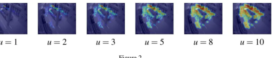
. (3)Fig. 2 shows examples of hot zone maps produced from the same heat values, but different values of parameter u. It should be noted that using u > 1 leads to a heat intensification effect, which allows lower visiting frequencies to be more noticeable. The left most picture shows a hot zone map without intensification (u
= 1). Without intensification, only the most frequently visited area, which is around cashier counter, is noticeable. This is trivial and provides virtually no marketing insight. With different degrees of intensification, the second most and other less frequently visited areas can be identified and examined, as shown in other pictures (u = 2, 3, 5, 8, 10).
This is a figure example:
Figure 2
Hot zone maps at various intensities
4 Integration of Multiple Cues
A classical object detection approach relies only on evaluating visual features containing in a window. Window is a very limited focal image area, compared to
an entire image frame. Complementarily, contextual information can provide important cues for visual perception, especially when image quality is poor [2].
Contextual information can be in many forms. Torralba [1] used a visual features of an entire scene as contextual information.
The notion of contextual information is based on a single frame detection. This study uses a term “additional cue” for a broader notion that also accommodates any useful addition for either a single frame or a video setting. For example, for video analytics, we may be able to use a state-based cue, such as frame continuity that a location of a customer in a subsequent frame is likely to appear near the one of its previous frame. The notion also can accommodate prior knowledge, such as an awareness of an entrance or an exit, where a customer can appear or disappear regarding frame continuity. This example of prior knowledge can provide relaxation on the state-based cue. Although our notion of additional cues initially developed based on additional information, it can be extended to integrate results from many decisive models. For example, a main cue may be drawn from a generic classifier, while an additional cue could be from a task-specific classifier.
This allows a local task-specific adjustment to a global generic inference system, which may be available off-the-shelf.
A simple integration scheme is derived based on a probabilistic approach. It follows an approach of Torralba [1]’s contextual priming with two major distinctions. Firstly, it is generality of a notion of an additional cue. Secondly, we relax probabilistic relation to explicitly distinguish two main components, a generic object detection model and a local characteristic model. This explicit discernment allows utilization of a well-trained generic object detection model with an enhancement tailored for a specific task. This approach aligns with an enticing concept of transfer and hierarchical learning. A classical object detection counts on a classifier to evaluate a set of visual features inside a window and determine if the window contains an object. A probabilistic approach is either to directly determine the likelihood that an object of interest is present or determine it through a generative model P(O|M) = P(M|O) P(O)/P(M), where P(O|M) is a conditional probability density function (PDF) of presence of the object O given a set of main features M. Since P(M) does not have any effect on an object inference and it is difficult to determine, it is omitted and the relation is left to P(O|M) P(M|O)·P(O).
Given that additional cue A is available, the presence of the object can be determined with the likelihood P(O|M,A). Applying Bayes’s rule, we get P(O|M,A) = P(O, M, A)/P(M,A) = P(M,A|O) P(O)/P(M,A). Denominator P(M,A) does not have any effect on the final decision, the likelihood can be written as, P(O|M,A) P(M,A|O)·P(O). Given training data, P(M,A|O) can be estimated.
Choices of estimating models are plentiful, e.g., Gaussian Mixture Model (GMM) and Expectation-Maximization method (EM), Self Organizing Map (SOM) and Artificial Neural Network (ANN), and, for a small set of data, Kernel Density Estimation (KDE).
With Bayes’ product rule, we also can write P(O|M,A) P(A|M,O)·P(M|O)· P(O).
This expression distinguishes a generic model P(M|O) and a local characteristics P(A|M,O). A generic model is a function of only primary information M. This modularization allows a use of an available good generic model with its adjustment to local characteristics. This may be interpreted as a local adjustment to exploit specific aspects in order to fine tune the combination to better fit a particular task. However, PDF P(A|M,O) is difficult to estimate. One possible remedy is to relax P(A|M,O) with an assumption that primary and additional cues are independent. That is, P(A|M,O) ≈ P(A|O), which leads to P(O|M,A) P(A|O)·P(M|O)·P(O). Both P(A|O) and P(M|O) can be estimated efficiently based on training data. Both P(A|O) and P(M|O) require generative models. An equivalent form for a main discriminative model is P(O|M,A) P(A|O)·P(O|M).
Term P(M) is also omitted here for the reasons discussed earlier. Similarly, when additional discriminative model is easier to acquired, the expression can be manipulated to P(O|M,A) P(O|A)·P(O|M)/P(O). The term P(O) can be simply estimated by No/N, where No is a number of windows containing the object and N is a number of all windows in a training set. Given such relation, define a decision score
) ( ˆ )
( X f X
f
s
d
a
m , (4)where fa() and fm() are score functions related to P(O = +1|A = Xˆ) and P(O = +1|M = X), respectively. Vectors X and Xˆ represent main and additional cues, respectively. The integrated model predicts a positive window class when sd > τ, otherwise it predicts a negative class. Parameterτ is a user specified threshold.
5 Experiments
Our system was built as the pipeline discussed in §3. The integration was meant for detection decision (Window Classification stage, Fig. 1). Our experiments were designed to demonstrate potential of the integration framework. Four treatments were examined. Three of them were represented by detectors of the same type, but trained on different datasets. The three datasets are a generic dataset, a task-specific dataset, and a combining dataset. These generic and task- specific notions were to simultaneously examined as another goal. That was to figure out how a local task specific cue could be used to enhance a generically well-tuned detector, so that the resulting model could perform better on a specific task without having to rebuild everything from scratch. A generic dataset, denoted
“Gdataset,” acquired data from Inria person dataset [22]. A task-specific dataset, denoted “Tdataset,” acquired data from a retailer video dataset (details discussed later). The third set, denoted “GT,” was a combination of both G and T datasets.
The treatments or models trained on G, T, and GT datasets were referred to as G,
T, and GT, respectively. The last treatment, denoted “G+AT”, represented a detector built on the integration framework with G model as its main cue and T model as its additional cue. Our experiment used 1/{1+exp(−s)} for score functions, fa(·) and fm(·) in Eq. 4, where s was s/smax when s was SVM decision score (Eq. 1) and smax was the maximum decision score.
G dataset was comprised of 2,416 positive, 4,872 negative, and 1,000 hard negative examples1. T dataset had 80 positive, 315 negative, 141 hard positive, and 582 hard negative examples. Video data recording activities in a retailer store, donated by our funder, was used for both training (as T dataset) and evaluation. A total of 20 video clips, each lasted about 30 sec. to 3 min., were separated into 15 and 5 clips for training and evaluating sets, respectively. Image frames were captured from video clips at a rate 1:30, which made it 1 frame/sec. All frames were 704x576-pixel RBG-color images. A region of interest (ROI) is defined to be an area of 250x150-pixel around a store entry. Each ROI was processed in 3 scales, 0.86x, 1x (original scale), and 1.2x. Windows were sampled by sliding window scheme at a window size of 64x128 pixels and step sizes of 4 in both x- and y-directions. Each window was passed through window classification process, which was central to our investigation, before gone through redundancy removal at an overlapping ratio over a threshold of 0.5.
All models, G, T, and GT, were HOG-based radial-basis SVM classifiers, but trained with three different datasets, as mentioned earlier. HOG features were computed with 9 orientations, cells of 8x8 pixels, and blocks of 2x2 cells. The SVM model was set with parameters C=10.0 and radial basis γ = 0.1. Detection performances, miss rate (MR) and false positive per window (FPW), of all treatments were evaluated against ground truth of the evaluation set of the retailer video data. The evaluation set contained 609 image frames.
It was worth emphasizing that treatment G was our implementation intended to replicate a classic Dalal-Triggs human detection [22]. Treatment G used Dalal- Triggs method and was trained with the same Inria person dataset. There were only two major differences. Firstly, SVM was trained on a smaller number of examples in order to mitigate a memory issue. Secondly, our implementation of HOG did not have a downweighing mechanism for pixels near the edges of the block, which Dalal and Triggs reported to contribute to only about 1%
improvement. However, it should be emphasized again that our study was not proposing a competing method against a classic Dalal-Triggs human detection
1 Hard negative examples are negative examples that were incorrectly classified by a simple classifier. We identified such examples in our preliminary study by applying a classifier trained with regular positive and negative examples on a set of negative examples. Then, negative examples that were incorrectly classified were hand-picked to be the hard-negative examples. Due to our memory limitation, we had to hand- picked negative examples that look distinct, so that they would be beneficial in a training process, while did not exhaust our computer memory.
[22]. Our framework was proposed as an approach to extend any object detection method, not limited to only Dalal-Triggs method [22]. Classical Dalal-Triggs schemes, mainly employing HOG features and SVM, were extensively used in all of our four treatments. They were to represent a generic detector, a task-specific detector, a conventional combined detector, and a combined detector based on our proposed framework.
Figure 3
Detection performances in MR-FPW plots: (a) all treatments and (b) treatments T and G+AT in a closer view.
Fig. 3a showed MR-FPW plots of 4 treatments. Treatment G+AT apparently outperformed treatments G and GT, but comparison between treatment G+AT and T was better seen in Fig. 3b, where treatment G+AT was shown to perform slightly better than treatment T. At FPW of about 0.0001, treatments G, T, GT, and G+AT delivered MRs at 0.507, 0.184, 0.263, and 0.106, respectively. That is, the integration framework showed 42% improvement over treatment T, the best performing treatment without the framework.
Discussion and Conclusions
The result shows promising potential of the framework. An integration of a task specific model to a generic model clearly improves over a generic model. This improvement is emphasized, since the integration also outperforms the model with a combining datasets. Therefore, this approach shows a benefit over simply combining datasets. Excluding the integration, model T outperforms the other two models. For model G, the explanation is obvious, but for model GT, which also has T dataset in its training, the explanation lies in the proportion of the training data. Generally, generic data is easier to be acquired than task-specific data is.
That reflects in sizes of training data. Here, sizes of G dataset to T dataset is 7.4:1.
This large difference may weigh down inference from T dataset excessively.
Building separate models and integrating them later with the integration framework allow some distinct characteristic inference of minority to prevail, while still retain principal values of the global majority. Those retaining global gumptions are those that are indispensable, which in turn deliver as an improvement seen over other models, including a task specific model. Our
findings are only preliminary and it requires a more thoroughly investigation to realize implication of this framework, as a key to tweak a global inference system with a local sense, as an ensemble of various models, as a fusion of different sources of information, or as a mélange of models and cues. Regarding worth investigating cues, specific characteristics of customers, e.g., constantly moving nature and common trajectory, frame continuity, and possible locations on a scene seem to be able to provide promising cues. Customer trajectory and locations may also provide a key to distinguish a high-level deduction, such as recognition of the difference between staff and customers. Frequently visited locations, conventionally an end result, itself can be fed back in the pipeline and used to deduce likeliness of presence of customers to improve detection quality, which in turn results in more accurate frequently visited locations. Customer trajectory is interesting as a propitious cue and as insightful visualization for understanding customer behavior. For customer behavior analysis via video analytics, issues of distortion and an application of object tracking appear worth prioritizing.
To summarize, this article provides a detailed discussion on an entire procedure for customer analysis via video analytics, as well as demonstrates potential of the integration framework for customer detection.
Acknowledgement
The authors appreciate Betagro Co.Ltd. for valuable data and funding our study and E-SAAN Center for Business and Economic Research (ECBER), Khon Kaen University for initiating and facilitating the cooperation.
References
[1] Torralba, A. “Contextual priming for object detection”, International Journal of Computer Vision 53(2), 169–191 (2003).
[2] Mottaghi, R., Chen, X., Liu, X., Cho, N.-G., Lee, S.-W., Fidler, S., Urtasun, R., and Yuille, A., “The role of context for object detection and semantic segmentation in the wild,” in Proc. IEEE Conf. Comput. Vis. Pattern Recog., 2014.
[3] Popa, M.C., Rothkrantz, L.J.M., Yang, Z., Wiggers, P., Braspenning, R.
and Shan, C., “Analysis of shopping behavior based on Surveillance System,” in Proc. IEEE Conf. Systems, Man, and Cybernetics (SMC), 2010.
[4] Popa, M.C., Rothkrantz, L.J.M., Shan, C., Gritti, T., and Wiggers, P.,
“Semantic assessment of shopping behavior using trajectories, shopping related actions, and context Information,” Pattern Recognition Letters 34(7), pp. 809–819 (2013).
[5] Connell, J., Fan, Q., Gabbur, P., Haas, N., Pankanti, S., and Trinh, H.,
“Retail video analytics: an overview and survey,” Proc. SPIE 8663, 2013.
[6] Jing, G., Siong, C.E., and Rajan, D., “Foreground motion detection by difference-based spatial temporal entropy image,” IEEE Region 10 Conference (TENCON), vol. A, pp. 379–392, 2004.
[7] Tang, Z., and Miao, Z., “Fast background subtraction and shadow elimination using improved gaussian mixture model,” IEEE International Workshop on Haptic Audio Visual Environments and Their Applications, pp. 38–41, 2007.
[8] Benenson, R., Omran, M., Hosang, J., and Schiele, B., “Ten years of pedestrian detection, what have we learned?,” European Conference on Computer Vision (ECCV), 2014.
[9] Dollar, P., Wojek, C., Schiele, B., and Perona, P., “Pedestrian detection: an evaluation of the state of the art,” IEEE Trans. Pattern Analysis and Machine Intelligence, vol. 99, 2011.
[10] Hosang, J., Benenson, R., and Schiele, B., “How good are detection proposals, really?,” British Machine Vision Conference (BMVC), 2014.
[11] Ullman, S., Assif, L., Fetaya, E., and Harari, D., “Atoms of recognition in human and computer vision,” Proc. Natl. Acad. Sci. USA 2016.
[12] Yang, B., Yan, J., Lei, Z., and Li, S. Z., “CRAFT objects from images,”
CVPR 2016.
[13] Morre, O., Veillard, A., Lin, J., Petta, J., Chandrasekhar, V., and Poggio, T., “Group invariant deep representations for image instance retrieval,”
Journal of Brains, Minds, and Machines 43, 2016.
[14] Yilmaz, A., Javed, O., and Shah, M., “Object tracking: a survey,” ACM Computing Surveys 38(4), 2006.
[15] Comaniciu, D., Ramesh, V., and Meer, P., “Real-time tracking of non-rigid objects using mean shift,” IEEE Conference on Computer Vision and Pattern Recognition, vol. 2, pp. 142–149, 2000.
[16] Chan-Hon-Tong, A., Achard, C., and Lucat, L., “Simultaneous segmentation and classification of human actions in video streams using deeply optimized Hough transform,” Pattern Recognition 47(12), pp. 3807–
3818, 2014.
[17] Pereira, E.M., Ciobanu, L., and Cardoso, J.S., “Context-based trajectory descriptor for human activity profiling,” IEEE International Conference on Systems, Man, and Cybernetics (SMC), pp. 2385–2390, 2014.
[18] Yu, J., Jeon, M., and Pedrycz, W., “Weighted feature trajectories and concatenated bag-of-features for action recognition,” Neurocomputing 131, pp. 200–207, 2014.
[19] Ko, T. “A survey on behavior analysis in video surveillance applications,”
Video Surveillance, Prof. Weiyao Lin (Ed.), InTech (2011), DOI:
10.5772/15302.
[20] Szegedy, C. , Liu, W., Jia, Y. , Sermanet, P., Reed, S., Anguelov, D., Erhan, D., Vanhoucke, V., and Rabinovich, A., “Going deeper with convolutions,” IEEE Conference on Computer Vision and Pattern Recognition (CVPR) 2015.
[21] Dollar, P., Belongie, S., and Perona, P., “The fast pedestrian detector in the west,” BMVC 2010.
[22] Dalal, N.andTriggs,B.,“Histograms of oriented gradients for human detection,” in Proc. IEEE Conf. Comput. Vis. Pattern Recog., 2005.
[23] Walk, S., Majer, N., Schindler, K., and Schiele, B., “New features and insights for pedestrian detection,” IEEE Conf. Computer Vision and Pattern Recognition, 2010.
[24] Viola, P. and Jones, M., “Rapid object detection using a boosted cascade of simple features,” in Proc. IEEE Conf. Comput. Vis. Pattern Recog., 2001.
[25] Fei-Fei, L., and Perona, P., “A bayesian hierarchical model for learning natural scene categories,” Computer Vision and Pattern Recognition, 2005.
[26] Felzenszwalb, R., McAllester, D., and Ramanan, D., “A discriminatively trained, multiscale, deformable part model,” IEEE Conference on Computer Vision and Pattern Recognition (CVPR), 2008.
[27] Malisiewicz, T., Gupta, A., and Efros, A. A., “Ensemble of exemplar- SVMs for object detection and beyond,” ICCV 2011.
[28] Cortes, C. and Vapnik, V., “Support-vector networks,”Machine Learning, 20, pp. 273–297 (1995).
[29] Chang, C.-C. and Lin, C.-J., “LIBSVM : a library for support vector machines,” ACM Transactions on Intelligent Systems and Technology, 2(27), pp. 1–27, (2011).
[30] Milgram, J., Cheriet, M., and Sabourin, R., “One against one or one against all: which one is better for handwriting recognition with SVMs?,”10th International Workshop on Frontiers in Handwriting Recognition, 2006, La Baule (France), Suvisoft.
[31] Canny, J., “A computational approach To edge detection,” IEEE Trans.
Pattern Analysis and Machine Intelligence, 8(6), pp. 679-698, 1986.
[32] Bishop, C., Pattern Recognition and Machine Learning. Springer, 2006.
[33] van der Maaten, L.J.P. and Hinton, G.E., “Visualizing high-dimensional data using t-SNE, ” Journal of Machine Learning Research, 9, pp. 2579- 2605, 2008.
Appendix: Multivariate Analysis
Means and variances of all datasets are shown in Figure A.1. In Figure A.1 (a), a mean of positive examples resembles a rough outline of a standing human. A mean of negative examples from G and T datasets looks like a simple gray patch.
This shows a well balance of variety of negative examples that are averaged to medium values throughout every pixel. Although a mean of hard positive examples from T dataset still resembles a rough outline of a human, it is less noticeable than those of regular positive examples. Hard positive examples from G datasets are excluded from our experiments or analysis for an economical reason. A mean of hard negative examples from T dataset vaguely resembles an area in the store where the classifier is often confused. A variance of hard negative examples from G datasets reveals a barely noticeable trace similar to an outline of human’s head and shoulder, which may be a reason that makes those examples difficult to classify. There is no sign of this trace in a variance of regular negative examples. A variance of hard negative examples from T datasets also reveals a lighter spot in the middle of the area. This high variation coincidentally locates around the middle of the area where critical classification is supposedly to take place. Therefore, it contributes to confusion and consequently makes those hard negative examples difficult to classify.
While human perceives each image patch effortlessly, a classifier takes each 64×128 pixel color image as a vector of 24576 values. Figure A.1 (b) shows means of all datasets as series of pixel-intensity values. Processing directly on this highly dimensional information requires a considerable amount of computing resources. A general approach is to convert the high-dimension data to more manageable lower dimension form. Our study employs Histogram of Oriented Gradient (HOG) [22] to map from 24576-dimension data to 3780-dimension HOG features. Figure A.1 (c) shows means of HOG features of all datasets. It should be noted that a mean of regular positive examples looks distinguishable from a mean of regular negative examples regardless of whether it is G or T dataset. However, patterns of hard examples are less distinguishable: a mean of hard negative examples from G dataset looks similar to the one of positive examples.
Examination of correlation, clustering, and visualisation of data with high dimensionality is less straightforward, but it can be mitigated using dimension reduction projection, e.g., t-SNE [33]. Figure A.2 shows scatter plots based on t- SNE projection from high dimensional datapoints onto a two-dimension space.
Since a mechanism of t-SNE is to project high dimensional datapoints onto a lower dimensional space such that a projected relative distance between similar datapoints is preserved, while a projected relative distance between dissimilar datapoints is allowed to have a higher degree of relaxation. Specifically, given datapoints in high dimensional space {x1,x2,···,xN} and xi ∈ RD, t-SNE is to find corresponding datapoints in low dimensional space {y1,y2,···,yN}, yi∈ Rd, and d <<
D. That is, {y1*,y2*,···,yN*}=argminy1,y2,···,yNiji pij log(pij/qij). A degree of relative similarity between high-dimension datapoints i and j is defined as pij = (pj|i +
pi|j)/(2N), where pb|a = (exp{-||xa-xb||2/2i2})/(ca exp{-||xa-xc||2/2i2}) and i’s are user specific parameters, called “perplexity.” A degree of relative similarity between low-dimension datapoints i and j is defined as qij = (1+||yi-yj||2)-1/ klk
(1+||yk-yl||2)-1. Problem formulation of t-SNE directly enforces that projections of similar datapoints must be projected onto close locations. It does not enforce the projections of dissimilar datapoints in the same degree. Distance between two dissimilar datapoints is indirectly enforced through mechanism of relativity. That is iji qij = 1, therefore when a projected distance between two dissimilar datapoints is too small, the corresponding projected relative similarity qij of those two dissimilar datapoints will be too large in the expense of that other projected relative similarities including the ones corresponding to similar datapoints will be too small. Consequently, that reflects to the objective function through too large values of terms corresponding to similar datapoints and the process of minimization will regulate to discourage projecting two dissimilar datapoints onto nearby locations.
Regarding t-SNE projections of original and HOG features (Figure A.2), HOG features do not seem to help much in term of data separation. The scale of Figure A.2 (a) may make it appear less separable than Figure A.2 (b), however, after a close investigation the t-SNE projection of original datapoints do not appear to be less separable than the t-SNE projection of HOG-mapped datapoints. At this point, an obvious advantage of using HOG features seems to be putting a number of dimensions down to a manageable size.
Figure A.1
Multivariate analysis of the datasets: (a) mean and variance of pixel intensities in each training dataset, presented as color images (each has 64x128x3 pixel intensities); (b) mean of pixel intensities in each training dataset, presented as a series of pixel intensities (each series has 24576 values); and (c) mean of HOG features in each training dataset. HOG scheme reduces dimensionality from 24576 of original pixel intensities to 3780 of HOG features. Acronyms “G”, “G Hard”, “T”, and “T Hard” indicate association to G dataset, hard examples from G dataset, T dataset, and hard examples from T dataset, respectively. Words “Positive” and “Negative” indicate association to positive examples and negative examples, respectively.
Figure A.2
Scatter plots of t-SNE projections of (a) original datapoints and (b) HOG-mapped datapoints.
Perplexity σi = 10 for all i’s. In order to mitigate memory issue, 50 representative points of each category are used instead of real datapoints. Representative points are centroids of clusters based on K- Means clustering. Symbols ‘G+’, ‘T+’, ‘TH+’, ‘G-’, ‘GH-’, ‘T-’, and ‘TH-’ indicate representative points for positive examples of G dataset, positive examples of T dataset, hard positive examples of T dataset, negative examples of G dataset, hard negative examples of G dataset, negative examples of T dataset, and hard negative examples of T dataset, respectively. (The image is best viewed in colors.)