Changes in Ultrasound Signals and Transducer Impedance for Imaging and Characterization

(1)

Changes in Ultrasound Signals and Transducer Impedance for Imaging and Characterization

Gergely Cs´ any

Theses of the Ph.D. Dissertation

Supervisor: Dr. Mikl´ os Gy¨ ongy

P´ azm´ any P´ eter Catholic University Faculty of Information Technology and Bionics

Roska Tam´ as Doctoral School of Sciences and Technology

Budapest, 2019

(2)

(3)

1 Introduction

A brief introduction to ultrasound technology

Ultrasound technology is a continuously developing, wide and diverse, exciting field of engineering. Among the diverse application fields, it is commonly used in clinical investigations and therapy (being used in around 20–25% of clinical imaging ex- aminations [6]). Ultrasound imaging– as a subfield – uses high frequency mechanical waves for localizing and characterizing objects or edges of objects containing ultrasound scatterers from which these waves reflect, inside media in which the waves are able to propagate. By definition,ultrasoundcan be any mechanical wave with a frequency above 20 kHz (frequencies not generally perceptible to the human ear) [7]. However, for imaging, significantly higher frequencies are tipically used (∼MHz range for acceptable resolution in medical imaging) [8, 9].

The devices able to convert electrical signals into mechanical waves and vice versa – being the pulsers and receivers of ultrasound – are called transducers [10]. Ultrasound images created using the common “pulse-echo” method are always built up from 1-D data. Dimension incrementation is achieved by some type of scanning. Scanning can be realized either by physically moving the transducer over the spatial region of interest or by applying several transducer elements appropriately arranged in space for electronic scanning (in which scanning is controlled electron- ically, without physical motion over the region of interest) [11].

(4)

Challenges in ultrasound relevant to thesis

The research presented in this work focuses on three different fields of ultrasonics. One of these fields is the characterization of transducers and estimation of their acoustic output with transducer models and specific measurements. Another area is in image data processing and within that, the quantification and visualization of indirectly present properties of these data. The third field of focus is in the creation of images with novel scanning techniques exploiting inherent information from the ultrasound pulse-echo signals.

Challenges in these fields for which the present work aimed to provide solutions are described below, followed by a brief sum- mary highlighting the intersection of the fields from the aspect of the present research.

Transducer characterization

Parameters defining safety of ultrasound transducers are measured usually by using either a hydrophone measurement system or a radiation force balance (RFB) [12, 13]. However, draw- backs for using such instruments are the difficulty in measuring high pressures, the time for the setup of field scans required for pressure measurements and power calculation (hydrophone systems) or the relatively high cost (7–24k USD) for specific- purpose devices (RFB). A method of rapidly testing transducers in a cost-effective manner, using otherwise multi-purpose standard laboratory equipment, may be useful in several use cases, including safety testing for biomedical applications [13].

The total power dissipation of a transducer is due to both electrical and acoustical losses. There exist methods using equivalent circuit models of transducers for a full description of their electrical and acoustical behaviour [14,15] – the most popular one

(5)

of such models is the KLM model [16]. However, these methods require extensive knowledge of transducer parameters [17] that are not necessarily available when testing. There exist works using simpler models of transducer systems [19] and methods based on electromechanical impedance measurements only [18], but have not been used for characterizing the transducer itself and its acoustic output, to the knowledge of the author.

Quantification of dynamics in a temporal ultrasound data sequence

Physical changes examined by ultrasound signals are usually interpreted and quantified by the commonly used Doppler techniques [8, 9]. These techniques are designed for moving tissue for typical image frames of less than 1 second. However, they are inapplicable for slow, long-term changes occurring in time frames of minutes, hours or of even longer time. There is a challenge in characterizing these changes with techniques relying on a completely different basis.

As described by Abbey et al. [20], comparing images recorded in the same spatial frame, at different moments in time, makes it possible to differentiate between (static and dynamic) components of the imaged object, based on signal statistics. The contribution of static scatterers to the overall decorrelation signal (comparing similarity of the images of the temporal image sequence) is constant. Contribution of dynamic scatterers to the overall correlation is decaying in time – it is assumed to show an exponential decay. The third component is noise (arising from data acquisition), which is assumed to be totally uncorrelated in time, so that its decorrelation component has the form of a Dirac delta function. The outlined component analysis of decorrelation functions is a promising basis for solving the above challenge.

(6)

Scanning using data-based position estimation in spa- tial ultrasound data sequence

Dimension incrementation of ultrasound images can be achieved by either electronic or mechanical scanning. Electronic scanning (using multi-element transducer arrays) is commonly used because of the great advantages of precise location information for each scan frame and of the capability of achieving high frame rates, however, such transducers can be realized at the cost of complex electronics and high costs of manufacturing, especially for higher (∼20 MHz) frequencies [11, 21]. In conventional mechanical scanning, either a motorized system is used – with increasing cost, complexity, and power consumption while reducing reliability [22] – or freehand scanning is performed with the use of position sensors, usually suffering from some combi- nation of issues including limited position accuracy, latencies in either position sensing or ultrasound data recording, or limita- tions on the scanning path that can be covered [23].

A potential alternative using information only of the data themselves for position estimation – taking advantage of the speckle pattern (interference caused by interaction of the ultrasound field and the scatterers) via correlation calculations – has been emerging recently in 3-D ultrasound technology [11]. How- ever, there are open questions such as how general these methods are to different tissues or transducer types; or can the ‘calibration curve’ (describing the one-to-one correspondence of distance and correlation) of these methods be estimated without assum- ing fully developed speckles and without using very specific or complicated models [24–27]. Furthermore, to the knowledge of the author, there is a gap in using such data-based methods for 1-D to 2-D scanning. Moreover, a need for a simple, real-time data-based scanning method arises in contrast to currently used

(7)

offline methods [28–31].

Challenges in dermatological ultrasonography

One of the most common cancers in the developed world is skin tumors [32]. Early differential diagnosis of skin cancer is crucial for better survival [33]. Ultrasound images are able to offer valuable additional information to standard dermato- scopic images about the type of skin lesion, non-invasively [34].

The penetration depth of ultrasound waves is inversely, but image resolution is directly proportional to the frequency of the waves [10]. Skin examination needs relatively high (∼20 MHz) frequency ultrasound imaging devices that are currently unavail- able for wide-spread, point-of-care use in dermatology.

Intersection of the above fields

The aspect from which the three fields of research were inter- connected in this work is: signal changes. Changes in electrical impedance signals of transducer systems with varying load media were used for transducer characterization. Temporal changes in sequences of ultrasound images were exploited by using correlation calculations and curve fitting for quantification and visualization of scatterer dynamics in time. Lastly, the effects of spatial changes were investigated and exploited using correlation calculations in signals from varying spatial locations for the development of data-based scanning methods.

The findings of this work open the potential for a diversity of applications. In particular, an application of the spatial- correlation-based scanning method has been realized in the creation of a portable and cost-effective ultrasound device for skin examination, providing solutions for challenges in screening and treatment planning of skin cancer, as presented in the final chapter of this work.

(8)

2 New Scientific Results

Thesis I: Use of a generalized two-port network model of ultrasound transducers is proposed for estimating the acoustic power output of transducers from electrical impedance measure- ments with the transducer placed in 3 different materials. As compared with reference acoustic measurements performed us- ing a hydrophone system, the proposed method gave a consistent overestimation (within 34%) of acoustic power output for HIFU (high intensity focused ultrasound) transducers, showing that it can serve as a practical tool for ensuring transducer safety.

Corresponding publication: [1].

A schematic of the basic elements of a piezoelectric ultrasound transducer is shown in Figure 2.1. The transducer has been modeled by a relatively simple equivalent circuit model (see Figure 2.2). In this model, the ‘backing’ part of the ‘transmis- sion line’ from the commonly accepted ‘KLM model’ [16, 17] is treated as part of the ‘black box’ having two ports only: one for the electrical voltage (V1) and another for the ‘front acoustic load’ of the transducer, represented by an equivalent electrical voltage (V2). By measuring the electrical impedance changes of the transducer when placed in 3 different load media, parameters of the two-port network model can be estimated, yielding an estimate of the acoustic power output (and accordingly, of the electrical power consumption of the transducer).

(9)

Figure 2.1: Schematic of a single transducer element system, showing elec- trical connections, back and front acoustic loading, and electrical matching as an optional part of the network. V1 and I1 stand for the voltage and current at the electrical port of the transducer, while V2 andI2 represent the acoustic pressure and particle velocity of the front acoustic load, seen as a voltage and current, respectively, in the equivalent circuit model.

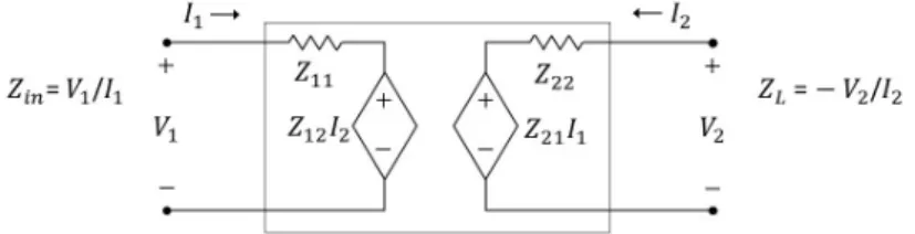
Figure 2.2: Schematic of the two-port network model with impedance param- etersZ11, Z12, Z21, Z22.ZLis the load impedance at port 2. The impedance measured at port 1 isZin.

A two-port network (Figure 2.2) is fully defined by 4 impedance parametersZ11, Z12, Z21, Z22[35,36], with state equations:

V₁ = Z₁₁I₁+Z₁₂I₂, (2.1) V₂ = Z₂₁I₁+Z₂₂I₂, (2.2) where V_n, I_n are the voltage at and current going into ports n ∈ 1,2, respectively. Placing an acoustic load ZL at port 2, the input impedanceZin=V1/I1 “seen” from port 1 is [37]:

(10)

Zin=Z11− Z12Z21

Z22+ZL

. (2.3)

With the assumption of reciprocity (Z12=Z21, generally true for circuits containing passive elements only and shown to be true for the KLM model [17]), the following system of equations can be solved for the parameter vector x(at any given frequency), with measurements of the input impedance Zin using at least three different acoustic loadsZL:

[Z_L,−Z_in,1]x = Z_inZ_L, (2.4) x = [Z₁₁, Z₂₂, Z₁₁Z₂₂−Z₁₂Z₂₁]⁰ . (2.5) Rearrangement of Eqs. (2.8) and (2.2), using also V₂ =

−ZLI2(see Figure 2.2), yields:

V₂= Z₁₁

Z21

1 + Z₂₂

ZL

−Z₁₂ ZL

−1

V₁, (2.6) Expressing all voltages in terms of their root mean squared (rms) value, the average power dissipated on the acoustic load is given by:

P_a =|V2|² ZL

=V₁² Z_L

Z₁₁

Z₂₁(ZL+Z22)−Z12

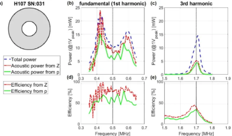
2 . (2.7) The method was tested for high-intensity focused ultrasound (HIFU) transducers (with 1.06, 3.19, 0.50, 1.70 MHz center frequencies) and compared with acoustic measurements performed by using a hydrophone system, as reference. Results are presented in Figures 2.3–2.4. The impedance-based method consis- tently overestimated the measured output, with errors of 17.0, 4.5, 21.8, 7.8% (for the above center frequencies, respectively).

(11)

Figure 2.3: Comparison of electrically estimated (from impedance “Z” mea- surements) and acoustically measured (estimated from acoustic pressure “p”

field measurements, as a reference) power outputs (1 V peak drive voltage) of the H-102 (SN: B-022) transducer. (a): Transducer surface schematic with the cutout. (b,c): Total (electric and acoustic) power and estimated and measured acoustic power. (d,e): Estimated and measured efficiency.

The dotted vertical lines indicate the centre frequency defined by the man- ufacturer at the fundamental and third harmonic resonances of the trans- ducer.

Figure 2.4: Comparison of electrically estimated and acoustically measured power outputs (1 V peak drive voltage) of the H-107 (SN: 031) transducer.

(12)

Electrical impedance measurements of a transducer in 3 propagation media is a relatively simple and quick method requiring standard laboratory equipment only. Therefore, with the results of consistent overestimation, the proposed method can be used as a simple, quick and potentially wide-spread means of ensuring transducer acoustic output falling within specified safety limits [13].

Thesis II: A method is proposed for quantitatively charac- terizing and visualizing the dynamic behavior of temporal changes in biological tissue by pixelwise decorrelation analysis of an ul- trasound image sequence, regardless of the rate of the changes (applying a PRF greater than the rate of changes to be observed).

The method was tested on post-mortem tissue effects, character- izing and mapping changes observed in time frames ranging from 100 to 5000 seconds at the level of small (∼800µm²) spatial ar- eas.

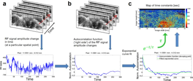
The proposed method is based on simple calculations of time constants for the exponential part of decorrelation functions calculated for raw ultrasound signal amplitude changes at a given spatial location (i.e. image pixel), see Figure 2.5. Quantification and visualization of the pixelwise dynamics in a temporal ultrasound image sequence is done with the following steps, according to the method. The amplitude change of a given image pixel in a temporal sequence of images is treated as a signal. Autocor- relation of this signal is calculated for positive time lags. An exponential curve is fitted to the initial, decaying part of the autocorrelation function. ‘Time constant’ parameterτis calculated from the fitted curve (f(t)) using the equations:

(13)

f(t) =Ae^−t/τ , (2.8) τ=−f(t)

f⁰(t). (2.9)

A spatial map of time constants (τ) visualizes the pixel-wise dynamics in an image sequence after calculatingτfor each pixel.

Figure 2.5: Method for calculating the map of time constants via exponential curve fitting to autocorrelation functions of pixel-wise temporal RF (raw radiofrequency) signal changes. (a)Observed RF signal amplitude change in time (for a given pixel);(b)Calculation of autocorrelation functions (for positive time lags);(c)Spatial map of time constants calculated from fitted exponential curves.

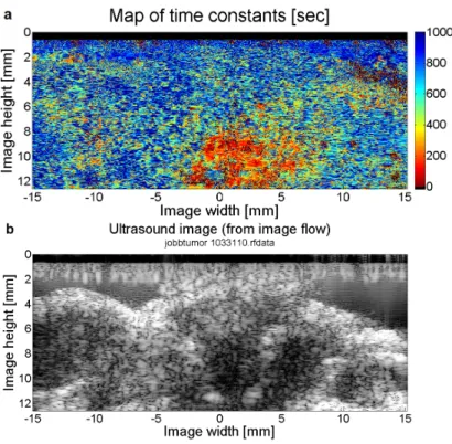
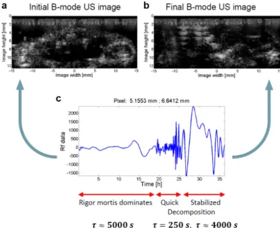
The method was successfully tested on investigating post- mortem tissue dynamics of mice (taking advantage of the lack of artifactual voluntary movements in these experiments and also making use of data from mice who did not survive experiments of a separate investigation). Quantitative results of dynamics characterization were in accordance with qualitative observations (on the ultrasound image sequences) both in short- (Figure 2.6) and long-term (Figure 2.7), in the ranges of 100 and 5000 seconds, respectively.

(14)

Figure 2.6: Spatial map of pixel-wise dynamics – characterized by time constants calculated from fitted exponential curves –(a) compared with a (typical) B-mode (brightness-mode) ultrasound image from an image se- quence of 53 minutes with 10.6 seconds temporal resolution(b). Warmer colors indicate smaller time constants – thus, a faster decay in correla- tion. On the other hand, colder colors refer to slower decay (with larger time constants) and indicate the places of (more) static scatterers. In order to achieve a better resolution for smaller time constant values, a limit of 1000 seconds was set for differences to be visualized.

Quantitative characterization and map-like visualization of dynamic changes can be useful in several application fields – with the great advantage of being independent of the time- course of the changes – including the monitoring of long-term biological phenomena such as response to therapy or slow blood perfusion in the capillaries or even in understanding the post- mortem redistribution of various drugs. Regarding industrial

(15)

Figure 2.7: Long-term tissue effects from an image sequence of 36 hours with 5 minutes temporal resolution. (a)First B-mode image from the image sequence (made at the time of death); (b)Final B-mode image from the image sequence (made 36 hours after death); (c)A sequence of temporal RF signal amplitude changes showing typical phases observed, together with calculated time constants for each phase, separately. The three separate phases are supposed corresponding to rigor mortis, relaxation of the corpse and advanced decomposition.

applications, an especially interesting potential application is the detection of signs of material fatigue (in materials being transparent to ultrasound).

(16)

Thesis III: A real-time spatial data-correlation-based free- hand scan conversion algorithm has been developed, using a fixed calibration curve for which robustness and simplified estimation process have been proven and from which an optimal range of input parameter ‘step size’ can be derived for the algorithm in the case of a specific imaging system.

Corresponding publications: [3] and [4].

Thesis III.a: A real-time freehand scan conversion algo- rithm has been developed for 2-D scan conversion using a single- element ultrasound transducer, being based on spatial correlation of data recorded.

Corresponding publications: [3] and [4].

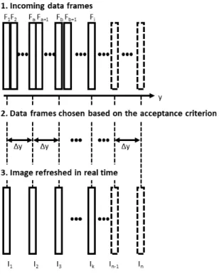
Sensorless freehand scanning has several advantages in ultrasound imaging such as cost-effectiveness and reduced complexity of the system. To compensate for distortions of the freehand movement, a data-based scan conversion method was introduced and generalized (for 1-D to 2-D scan conversion), estimating spatial distances based on a measure of correlation. The real-time algorithm uses a predefined image grid with a uniform inter-line distance. The defined distance corresponds to a certain correlation coefficient due to the calibration curve. Each incoming data frame is accepted into the image grid if it has the expected correlation coefficient with the last accepted J >= 1 data frames, otherwise it is rejected (Figure 2.8):

αi,k=

J

X

j=1

w(j, J)

ρI_k−j,F_i−ρ(j∆y)

< . (2.10) ρIk−j,F_i is the Pearson correlation coefficient of the actual incoming frameFi and a previously accepted frameI_k−j from the

(17)

predefined image grid of a grid distance ∆y. ρ(j∆y) is the ex- pected correlation coefficient from the calibration curve, which should be approximated byρI_k−j,F_i within an error of for acceptance (α). (w(j) are a set of weights for a window sizeJ.)

Figure 2.8: Schematic illustrating the concept of the proposed real-time data-based scanning method. The desired image grid is filled with data frames chosen based on an acceptance criterion, in real time [4].

The algorithm was tested for being able to generate an image from 1000 A-line frames in 345±132 ms (using MATLAB on a computer with Intel Core i5 processor, 8 GB RAM). For a dedicated architecture, with a 10-fold oversampling and a PRF

≥667 Hz, a scanning speed of≥20 mm/s is estimated.

The method can be applied in sensorless freehand scanning,

(18)

with special usage of applications in which cost-effectiveness, complexity, the need for eliminating mechanical motion elements or acoustic coupling is a major constraint while dimension incrementation (of images) is needed. Specific applications are in skin imaging and in high-frequency non-destructive testing.

Moreover, the method can also be applied for annular array transducers (providing high-quality and smooth focus at the cost of dimension incrementation) [38, 39].

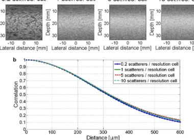
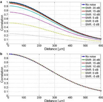
Thesis III.b: I showed that the calibration curve (reflecting spatial decorrelation) for data-based scan conversion is primar- ily a function of transducer characteristics (being less dependent on the examined media). The calibration curve was found to be robust enough for different scatterer densities (8.3×10⁻³ mean absolute error) and signal-to-noise ratios (1.0×10⁻³ mean abso- lute error for -5 dB SNR) for simulations presented in this thesis.

This result allows the use of the scan conversion algorithm on a wide variety of imaged media with a single transducer calibration.

The data-based scanning method ofThesis III.arelies on the one-to-one correspondence of the distance between two parallel data frames and their “similarity” measured by the Pearson correlation coefficient (for distances within transducer beamwidth and ideally in homogeneous fully developed speckle case, due to the literature [40, 41]). This distance-correlation correspondence is defined by the calibration curve (representing correlation as a function of distance).

As stated above, calibration curve was tested for different scatterer densities (Figure 2.9) and signal-to-noise ratios (Fig- ure 2.10), and found to be robust enough, with mean absolute

(19)

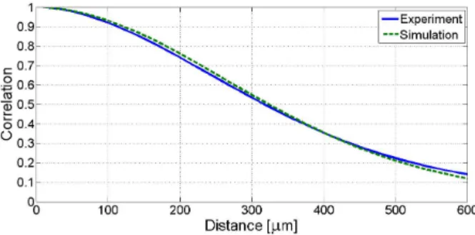
errors on the scale of 10⁻³ for both. Higher but still acceptable differences were found when comparing calibration curves obtained from simulated and experimental data: 1.19×10⁻² mean absolute error (Figure 2.11).

It was also presented that use of a fixed calibration curve compared to an adaptive calibration curve – taken from the literature [27] – gave similar accuracies in scan conversion (see Thesis III.d), with an average overlap of the accuracy ranges of 92.94% for simulations and 42.83% for experiments, for the data presented, while the proposed method using a fixed calibration curve had the great advantage of a 350-fold faster computation time.

Figure 2.9: (a) Simulated B-mode images and(b)calibration curves cal- culated from raw (RF) image data of homogeneous phantoms of 0.2, 1, 5 and 10 scatterers/resolution cell densities. The simulated ultrasound imag- ing system was a single element Olympus V317 transducer moved along the lateral dimension, collecting A-lines with an equal 10µm spacing.

(20)

Figure 2.10: Calibration curves calculated from simulated image data of homogeneous phantom (10 scatterers / resolution cell density, see Fig- ure 2.9.a) without noise and with additional (Gaussian random distribu- tion) noise according to 20 dB, 15 dB, 10 dB, 5 dB, 0 dB and −5 dB SNR. (a) Calibration curves are presented as calculated (containing also noise level information in initial decay). (b)Normalized calibration curves in order to make a visual comparison of the decay rate similarity for the curves.

Statement of this thesis confirms the robustness of the proposed method, eliminating the necessity for performing calibration on a wide variety of circumstances (at least of scatterer densities and noise levels).

(21)

Figure 2.11: Normalized calibration curve from experimental data (3% agar – 4% graphite homogeneous phantom) compared to calibration curve from simulated data (homogeneous phantom with 10 scatterers / resolution cell density).

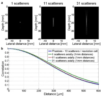
Thesis III.c: I found that for estimating the calibration curve, a few (31 in 1 mm distances for∼8 MHz transducer) scat- terers placed along the axis of ultrasound pulse-echo propagation and covering the axial region of interest are sufficient. This re- sult allows for calibration curve estimation calculations with the following advantages: a significant fastening of calibration curve calculation in simulations and a widening of possibilities for cal- ibration curve calculations based on phantom measurements.

A series of (odd numbers of 1–31) scatterers were placed with 1 mm distances (to avoid interference) covering the range of interest (for imaging with a∼8 MHz transducer) through an axial line, around the focus of the transducer.

The calibration curves calculated using these simple simulated phantoms were compared to the one obtained from fully developed speckle (FDS) simulation (10 scatterers / resolution cell from Figure 2.9), by calculating the mean absolute difference between the calibration curves compared (see Figure 2.12).

(22)

Figure 2.12: (a)Simulated B-mode images of 1, 11 and 31 scatterers (cor- responding to single focus point, depth of field and axial region of interest, respectively) placed around transducer focus with a uniform axial spacing of 1 mm. The imaging system simulated was the same as for Figure 2.9.

(b) Calibration curves calculated from raw (RF) image data of (a), and compared with the calibration curve calculated from simulated image of a FDS homogeneous phantom (10 scatterers / resolution cell density) as a reference (Figure 2.9).

The best correspondence was found for the phantom covering the same axial range as that of the FDS phantom, using 31 scatterers. The mean absolute difference for this pair of calibration curves was found to be insignificant, being only 6.9×10⁻³ in the case of the simulations presented. This result suggests the possibility for a simplified process of calibration curve estimation for single-element transducers. Using such simplified phantoms significantly reduces calculation time in simulations (simulated ultrasound image calculation took ∼10 seconds for 31 scatterers while taking ∼7.5 hours for FDS

(23)

phantom with 154 740 scatterers on a PC with Intel Core i5 processor, 8 GB RAM) and widens the field of feasible phantom manufacturing techniques for experimental calibration curve estimation (such that wire phantoms and 3-D printed phantoms become applicable).

Thesis III.d: I showed that there exists a range for image grid step sizes, within which the proposed scan conversion algo- rithm has optimal performance, and that the optimal step size can be determined from the calibration curve.

For quantitative analysis of the performance of the proposed scan conversion algorithm (seeThesis III.a), two error measures were used for position estimation errors. Bias error (eb) was used to describe the linear increase in error between the true (y_t) and desired (y_d) positions as a function of the desired position:

eb= arg min

e ky_t−ey_dk₂. (2.11) Ripple error (er) was used to measure the root mean square position error after correcting for bias:

er=ky_t/eb−y_dk₂. (2.12) When analyzing the proposed scan conversion algorithm in terms of the above position estimation errors, it was found that a range of image grid step sizes (being an input of the algorithm) exists in which both the bias and ripple errors are minimal. This led to the recognition that, for a specific transducer and calibration curve, a range of image grid step sizes can be determined using which optimal performance of the scan conversion algo-

(24)

rithm can be attained. The region is in correspondence with the slope of the calibration curve. The higher the slope (absolute derivative) is, the more likely optimal performance of position estimation will be achieved. In the cases of the experiments presented, bias and ripple errors were not exceeding 3.9% or 85.5µm, respectively for a wide range of image step sizes: 150–

350 µm (Figure 2.13). Worse performance was obtained with experimental data: < 15.4% absolute bias and < 1143.0 µm ripple, but still being optimal on the same range (Figure 2.14).

Figure 2.13: Position estimation errors (in green) for simulated data of a homogeneous phantom with FDS (10 scatterers/resolution cell) using (a) fixed and(b)adaptive calibration curves. Cumulative errors (bias)(left) and ripple errors(right)are presented for different step sizes (distances) of position estimation. The corresponding correlation values of the fixed calibration curve (obtained from the same phantom) are shown in blue.

(25)

Figure 2.14: Position estimation errors (in green) for experimental data of a homogeneous agar-graphite phantom using(a)fixed and(b)adaptive calibration curves. Cumulative errors (bias)(left)and ripple errors(right) are presented for different step sizes (distances) of position estimation. The corresponding correlation values of the fixed calibration curve (a version of the simulated phantom calibration curve, corrected for noise) are shown in blue.

Performance of the proposed algorithm using a fixed calibration curve has been compared to the performance of the same algorithm using adaptive calibration curve due to a method taken from the literature [27]. Position estimation errors were similar for the two methods, with 92.94% overlap of error ranges in average for bias and ripple errors in simulations, and 42.83%

overlap of error ranges in experiments (as an average of 62.28%

overlap for ripple errors and 23.39% overlap for absolute bias errors). The use of a fixed calibration curve was leading to slightly

(26)

higher absolute bias but lower ripple errors. Nevertheless, the main improvement of the proposed method using a fixed calibration curve is its running time: providing a 350-fold improvement in computational time (on the hardware mentioned in the discussion ofThesis III.a).

Direct application of Thesis III.d is the deduction of image grid step sizes to be used for a scanning system with a certain calibration curve.

(27)

3 Application of the Results

Cost-effective portable skin ultrasound imaging device

A particular industrial application of the data-based scan conversion method presented in Thesis III has been realized in the creation of a cost-effective portable ultrasound device for skin examination [5]. Imaging deeper structures of the skin (in addition to conventional dermoscopy examination) can provide extensive and crucial information for the diagnostics and treatment planning of various common and serious skin diseases (such as skin cancer) [34, 42]. However, the use of skin ultrasound examination has not been spread widely in dermatological practice yet, partially due to the high cost of multi-element transducers of a high enough frequency (∼20 MHz) needed for skin examination [21]. Using a single-element high-frequency transducer with the proposed data-based scan conversion method has been addressed in the present work to overcome this issue.

The device was built of commercially available components (including an Olympus V317 single-element, spherically focused ultrasound transducer) with a custom-designed plastic case cover, which has been designed to realize manual scanning without damaging the skin and with minimal usage of gel. Compo- nents of the device are shown in Fig. 3.1.

The device prototype and the algorithm were validated in a clinical study (with ethical approval OGY ´EI/16798/2017). 184 skin lesions have been examined at the Department of Dermatol- ogy, Venereology and Dermatooncology, at Semmelweis Univer-

(28)

Figure 3.1: Components of the portable, cost-effective skin imaging ultra- sound device prototype.

sity (Budapest, Hungary). Resulting ultrasound images of the portable device prototype have been compared to ultrasound images of a reference device (Hitachi Preirus with EUP-L75 linear array transducer) and with histopathological images of the same lesion (Fig. 3.2).

Performance of the real-time data-based scan conversion algorithm has been proved to be acceptable on in-vivo images of human skin tissue (Figure 3.3). Qualitative observations showed the clinically relevant information present on the resulting images, without significant distortions. Quantitatively, lesions with 0.7–5.5 mm (axial) thicknesses and 3.1–14.6 mm (lateral) widths, the mean absolute difference and standard deviation of measured dimensions on the portable device images as compared to those measured on corresponding reference images were 10.8 ±8.6%

in width and 8.6 ±6.7% in thickness (with the latter indicating the inaccuracy of the measurement itself).

(29)

Figure 3.2: Comparison of corresponding ultrasound images obtained with a commercial reference device (Hitachi Preirus with EUP-L75)(left)and those obtained with the proposed portable skin imaging device(middle)and of photographs taken of the slices used in histological examination(right) of certain lesions: melanoma (top), keratosis seborrhoica (middle) and basalioma(bottom).

Figure 3.3: In vivoultrasound images of a melanoma on a human sole(a) Ultrasound image obtained with the reference device using a linear array transducer. (b) Ultrasound image of the same lesion obtained with the portable device prototype using a single element transducer and the proposed scan conversion algorithm. (c)Set of data frames (A-lines scanned by the single element transducer) prior to scan conversion. Red lines indicate data frames accepted to the image grid (b) (with a grid distance of 305µm corresponding to a correlation coefficient of 0.5).

(30)

Other fields of application

The simple method of Thesis I for acoustic power estimation can be performed relatively quickly (within ∼15 minutes) and cost-effectively, using standard laboratory equipment and commonly available laboratory supplies (such as air, water and glycerine as the load materials). In this way, custom-designed transducers may be quickly tested during production without requiring a full characterization. Moreover, during manufacturing, all manufactured items may be tested without the need for random sampling. Lastly, a clinician may test the performance and safety of a transducer over time without requiring access to expensive equipment (even for the case of the portable skin ultrasound imaging device presented above).

The quantitative characterization and map-like visualization method for dynamic changes in an image sequence (Thesis II) can be applied in a broad range of applications in which pixel- wise dynamics in an image sequence are of interest and even in which changes occur over relatively large time-courses making conventional ultrasound Doppler techniques unusable. Some of the potential applications in biomedical ultrasonics (such as monitoring of long-term response to therapy or slow blood perfusion in the capillaries, or understanding the post-mortem redistribution of various drugs) and in material fatigue detection haves already been mentioned in Chapter 2.

Regarding the proposed real-time data-based scan conversion method (Thesis III), a specifically beneficial application would be the scanning with annular array transducers [38, 39]. Results ofTheses III.b–dcan be applied in the simplification of a robust calibration curve and scan conversion parameter estimation.

(31)

Acknowledgements

Despite having an extraordinary interest in dolphins and playing music seriously and enthusiastically since a very young age, I never thought of the field of ultrasound before as a potential field of my research and studies. Never before I met Dr.

Mikl´os Gy¨ongy. He was so convincing and I truly have learnt so many things from him which I admired such as consistency, predictability, effective and realistic planning of work in addition to his assertive communication, understanding and natural humility. I have gained skills in thinking as an engineer, in re- searching attitude, in industrial utilization of results and in the ins and outs of scientific publication, at his side. I am so grateful to him for his leading by example and for all of his guidance making this work possible.

I thank my collaborators, with special thanks to Dr. Klára Szalai, chief radiologist at the Department of Dermatology, Venereology and Dermatooncology of Semmelweis University (Budapest, Hungary). I am grateful to Prof. Dr. Tamás Roska, Prof. Dr. Sarolta Kárpáti and Prof. Dr. Miklós Sárdy for es- tablishing our collaboration with the dermatology clinic. I am grateful to Dr. Michael Gray, an excellent engineer from the BUBBL lab of the Institute of Biomedical Engineering, Depart- ment of Engineering, University of Oxford (Oxford, UK). His collaboration during the research presented in Thesis I was truly exemplary. I further thank Prof. Dr. Constantin-C. Coussios (my ‘grand-supervisor’), Dr. Lajos Balogh, Dr. Enikö Kuroli, Rita Mátrahegyi, Dr. Jeffrey Ketterling, Dan Gross, Krisztián Füzesi, Balázs Bajnok and Máté Kiss for their cooperation and contribution.

(32)

I am grateful to all of my teachers who guided me through my studies at Budai Ciszterci Szent Imre Gimnázium and at PPKE-ITK, with special thanks to Prof. Dr. Árpád I. Csurgay.

I am grateful to the directorate and administrative assistants of the doctoral school, in particular to Prof. Dr. P´eter Szolgay, Dr.

Kristóf Iván, Tivadarné Vida and L´ıvia Adorján.

I thank my longer term labmates, Janka Hatvani, Dr.

Krisztián Füzesi, Ákos Makra, Péter Marosán, Domonkos Csabai and Ádám Simon, for working together and for their impulses and helpfulness through the years.

I thank my fellow PhD students, with special thanks to Domokos Meszéna, Bertalan Kovács, Sándor Földi and Márton Hartdégen, my best friends, for sharing this journey and for the many memorable discussions, inspiration and encouragement.

I am extremely grateful to my family, with special thanks to my lovely wife, Mária Csány and parents, László Miklós Csány and Dr. Ragyiánó Rita Csányné and to my sister and brothers.

First of all, I am grateful to the Creator for hiding things to be discovered through science and for giving us thespirit to go after them, to discover them and to create new devices by invention.

The presented research was supported by grants KAP14–17 of Pázmány Péter Catholic University; János Bolyai scholarship of the Hungarian Academy of Sciences; grant PD 121105 of the Hungarian National Research, Development and Innovation Of- fice; Hungarian state funding EFOP-3.6.2-16-2017-00013, 3.6.3- VEKOP-16-2017-00002; and GINOP-2.1.7-15-2016-02201.

I thank Elsevier’s journal Ultrasonics for the

‘R.W.B. Stephens Prize’ I was awarded for my presentation at the 2017 International Congress on Ultrasonics (ICU2017); the Hungarian Dermatological Society (MDT) for ‘The Best Poster’

award of the 90th Congress of MDT (2017); and PPKE for the

‘PhD Excellence Scholarship’ (2015).

(33)

References

Publications of the author

[1] G. Cs´any, M. D. Gray, and M. Gy¨ongy, “Estimation of acoustic power output from electrical impedance measurements,” in Acoustics, Multidisciplinary Digital Publishing Institute, vol. 2, no. 1, pp. 37–50, feb 2020.

https://doi.org/10.3390/acoustics2010004

[2] G. Cs´any, L. Balogh, and M. Gy¨ongy, “Investigation of post- mortem tissue effects using long-time decorrelation ultrasound,”

Physics Procedia, vol. 70, pp. 1195–1199, aug 2015.

https://doi.org/10.1016/j.phpro.2015.08.257

[3] G. Cs´any, K. Szalai, and M. Gy¨ongy, “A real-time data-based scan conversion method for single element ultrasound transducers,”Ultrasonics, vol. 93, pp. 26–36, oct 2018.

https://doi.org/10.1016/j.ultras.2018.10.006

[4] M. Gy¨ongy andG. Cs´any, “Method for generating ultrasound image and computer readable medium,” Patent, Dec. 29, 2016, WO Patent Application 2016/207 673.

[5] G. Cs´any, K. Szalai, K. F¨uzesi, and M. Gy¨ongy, “A low-cost portable ultrasound system for skin diagnosis,” in Proceedings of Meetings on Acoustics 6ICU, vol. 32, no. 1, p. 020002. Acous- tical Society of America, mar 2017.

https://doi.org/10.1121/2.0000701

(34)

Other references

[6] C. R. Hill, J. C. Bamber, and G. R. ter Haar, “Physical principles of medical ultrasonics,” 2004.

[7] K. K. Shung and G. A. Thieme,Ultrasonic scattering in biolog- ical tissues. CRC Press, 1992.

[8] P. N. Burns, “Introduction to the physical principles of ultrasound imaging and doppler,” Fundamentals in Medical Bio- physics, 2005.

[9] T. L. Szabo,Diagnostic ultrasound imaging: inside out. Aca- demic Press, 2004.

[10] R. S. Cobbold,Foundations of biomedical ultrasound. Oxford University Press, 2006.

[11] A. Fenster, D. B. Downey, and H. N. Cardinal, “Three- dimensional ultrasound imaging,” Physics in Medicine & Bi- ology, vol. 46, no. 5, p. R67, 2001.

[12] R. C. Preston, Output measurements for medical ultrasound.

Springer Science & Business Media, 2012.

[13] A. Shaw and K. Martin, “The acoustic output of diagnostic ultrasound scanners,”The safe use of ultrasound in medical di- agnosis. 3rd ed. London: The British Institute of Radiology, pp.

18–45, 2012.

[14] T. F. Johansen and T. Rommetveit, “Characterization of ultrasound transducers,” in Proc. of the 33rd Scandinavian Sympo- sium on Physical Acoustics, 2010.

[15] J. L. San Emeterio and A. Ramos, “Models for piezoelectric transducers used in broadband ultrasonic applications,” in Piezoelectric Transducers and Applications. Springer, pp. 97–

116, 2009.

(35)

[16] R. Krimholtz, D. A. Leedom, and G. L. Matthaei, “New equivalent circuits for elementary piezoelectric transducers,”Electron- ics Letters, vol. 6, no. 13, pp. 398–399, 1970.

[17] S. Van Kervel and J. Thijssen, “A calculation scheme for the optimum design of ultrasonic transducers,”Ultrasonics, vol. 21, no. 3, pp. 134–140, 1983.

[18] V. G. M. Annamdas and C. K. Soh, “Application of electromechanical impedance technique for engineering structures: review and future issues,”Journal of Intelligent Material Systems and Structures, vol. 21, no. 1, pp. 41–59, 2010.

[19] E. B. Ndiaye, H. Duflo, P. Mar´echal, and P. Pareige, “Thermal aging characterization of composite plates and honeycomb sand- wiches by electromechanical measurement,”The Journal of the Acoustical Society of America, vol. 142, no. 6, pp. 3691–3702, 2017.

[20] C. K. Abbey, M. Kim, and M. F. Insana, “Perfusion signal processing for optimal detection performance,” in Ultrasonics Symposium (IUS), 2014 IEEE International. IEEE, pp. 2253–

2256, 2014.

[21] C. Liu, F. T. Djuth, Q. Zhou, and K. K. Shung, “Micromachin- ing techniques in developing high-frequency piezoelectric composite ultrasonic array transducers,”IEEE Transactions on Ul- trasonics, Ferroelectrics, and Frequency Control, vol. 60, no. 12, pp. 2615–2625, 2013.

[22] A. J. Medlin and A. J. P. Niemiec, “Scan line display apparatus and method,” Apr. 28 2011, uS Patent App. 12/674,007.

[23] M. A. Bahramabadi, “Sensorless out-of-plane displacement estimation for freehand 3D ultrasound applications,” Master’s thesis, Carleton University Ottawa, 2014.

[24] N. Afsham, M. Najafi, P. Abolmaesumi, and R. Rohling, “A generalized correlation-based model for out-of-plane motion estimation in freehand ultrasound,”IEEE Transactions on Med- ical Imaging, vol. 33, no. 1, pp. 186–199, 2014.

(36)

[25] F. Dong, D. Zhang, Y. Yang, Y. Yang, and Q. Qin, “Dis- tance estimation in ultrasound images using specific decorrelation curves,” Wuhan University Journal of Natural Sciences, vol. 18, no. 6, pp. 517–522, 2013.

[26] C. Laporte and T. Arbel, “Measurement selection in untracked freehand 3D ultrasound,” inInternational Conference on Med- ical Image Computing and Computer-Assisted Intervention.

Springer, pp. 127–134, 2010.

[27] A. H. Gee, R. J. Housden, P. Hassenpflug, G. M. Treece, and R.

W. Prager, “Sensorless freehand 3D ultrasound in real tissue:

speckle decorrelation without fully developed speckle,” Medical Image Analysis, vol. 10, no. 2, pp. 137–149, 2006.

[28] M. Li, “System and method for 3-D medical imaging using 2-D scan data,” Patent, Dec. 10, 1996, US patent 5,582,173.

[29] N. C. Kim, H. J. So, S. H. Kim, and J. H. Lee, “Three- dimensional ultrasound imaging method and apparatus using lateral distance correlation function,” Patent, Jan. 24, 2006, US patent 6,988,991.

[30] L. Y. Mo, W. T. Hatfield, and S. C. Miller, “Method and apparatus for tracking scan plane motion in free-hand three- dimensional ultrasound scanning using adaptive speckle correlation,” Patent, Jan. 11, 2000, US patent 6,012,458.

[31] C. Laporte, Statistical methods for out-of-plane ultrasound transducer motion estimation. McGill University, 2009.

[32] G. P. Guy Jr, C. C. Thomas, T. Thompson, M. Watson, G. M.

Massetti, and L. C. Richardson, “Vital signs: melanoma inci- dence and mortality trends and projections — United States, 1982–2030,” MMWR. Morbidity and mortality weekly report, vol. 64, no. 21, p. 591, 2015.

[33] American Cancer Society, “Key statistics for melanoma skin cancer,” https://www.cancer.org/cancer/melanoma-skin- cancer/about/key-statistics.html, Accessed: 2017 Dec.

(37)

[34] D. S. Rigel, J. Russak, and R. Friedman, “The evolution of melanoma diagnosis: 25 years beyond the ABCDs,”CA: a can- cer journal for clinicians, vol. 60, no. 5, pp. 301–316, 2010.

[35] W. H. Hayt, J. E. Kemmerly, and S. M. Durbin, Engineering circuit analysis. McGraw-Hill New York, 2002.

[36] A. S. Sedra and K. C. Smith, Microelectronic circuits. New York: Oxford University Press, 1998.

[37] W. Y. Yang and S. C. Lee,Circuit Systems with MATLAB and PSpice. John Wiley Sons, 2008.

[38] K. A. Snook, C.-H. Hu, T. R. Shrout, and K. K. Shung, “High- frequency ultrasound annular-array imaging. Part I: Array design and fabrication,” IEEE Transactions on Ultrasonics, Fer- roelectrics, and Frequency Control, vol. 53, no. 2, pp. 300–308, 2006.

[39] J. Hatvani, “Use of annular arrays in ultrasound imaging,” Mas- ter’s thesis, Pázmány Péter Catholic University, Faculty of In- formation Technology and Bionics, Budapest, Hungary, 2016.

[40] J. M. Thijssen, “Ultrasonic speckle formation, analysis and processing applied to tissue characterization,”Pattern Recognition Letters, vol. 24, no. 4-5, pp. 659–675, 2003.

[41] P. Hassenpflug, R. W. Prager, G. M. Treece, and A. H. Gee,

“Speckle classification for sensorless freehand 3-d ultrasound,”

Ultrasound in Medicine Biology, vol. 31, no. 11, pp. 1499–1508, 2005.

[42] E. Christensen, P. Mjønes, O. A. Foss, O. M. Rørdam, and E. Skogvoll, “Pre-treatment evaluation of basal cell carcinoma for photodynamic therapy: comparative measurement of tu- mour thickness in punch biopsy and excision specimens,” Acta Dermato-Venereologica, vol. 91, no. 6, pp. 651–655, 2011.