Changes in Ultrasound Signals and Transducer Impedance for Imaging and Characterization

(1)

Changes in Ultrasound Signals and Transducer Impedance for

Imaging and Characterization

Gergely Cs´ any

Supervisor: Dr. Mikl´ os Gy¨ ongy

P´ azm´ any P´ eter Catholic University

Faculty of Information Technology and Bionics

Roska Tam´ as Doctoral School of Sciences and Technology

A thesis submitted for the degree of Doctor of Philosophy

Budapest, 2019

(2)

Abstract

Three main topics are presented in this thesis. A method is proposed for esti- mating the acoustic power output of ultrasound (US) transducers based on electrical impedance measurements of the transducer loaded by (N=3) various propagation media. The method being based on a two-port network model of the transducer was compared with acoustic measurements for high-intensity focused ultrasound (HIFU) transducers at center frequencies of 1.06, 3.19, 0.50, 1.70 MHz, consistently overes- timating measured output with corresponding errors of 17.0, 4.5, 21.8, 7.8%. The results suggested a simple means of ensuring transducer acoustic output falls within specified safety limits.

A decorrelation ultrasound method is proposed for quantitatively characterizing dynamic changes on an ultrasound image sequence, based on the temporal decorrelation of signals coming from certain spatial locations. The method was tested on post-mortem tissue effects of mice. Quantitative results of dynamics characterization were in accordance with qualitative observations of the biological phenomena both in short- (∼100 s) and long-term (∼5000 s).

A real-time data-based scanning method is proposed for position estimation (PE) of ultrasound A-lines obtained via sensorless freehand scanning. Simulations and experiments showed the PE calibration curve to be robust enough for different scatterer concentrations, signal-to-noise ratios, and being predictable from a small number (31) of point scatterers, with ∼10⁻³ mean absolute errors. Use of a fixed versus an adaptive calibration curve gave similar PE accuracies with optimal performance for 150–350 µm scanning step sizes, and a 350-fold improvement in computation time.

Clinical images of skin lesions demonstrated the feasibility of the algorithm for real, non-homogeneous tissue. Application of the scanning method led to the creation of a portable and cost-effective skin examination US device, providing solutions for challenges in screening and treatment planning of skin cancer.

(3)

Declaration of original work used

Chapters 2–5 present the scientific work of the author published recently in peer- reviewed journals or in conference proceedings as follows. Chapter 2 is based on [1].

Chapter 3 is based on [2]. Chapter 4 is based on [3] and [4]. Chapter 5 is based on [5].

(4)

List of Figures

1.1 Schematic of the pulse-echo method. . . 5 1.2 Basic steps of signal processing for ultrasound A-lines. . . 7 1.3 Schematic showing the main components of a piezoelectric transducer. 14 1.4 Schematic illustrating the concept of electronic scanning. . . 16 1.5 Schematic illustrating the concept of mechanical scanning. . . 17 1.6 Schematic illustrating the concept of freehand scanning with a posi-

tion sensor. . . 18 1.7 Schematic illustrating the concept of freehand scanning without po-

sition sensors. . . 20 2.1 Schematic of a single transducer element system. . . 38 2.2 Schematic of the two-port network model. . . 38 2.3 Setup of the electrical impedance measurements and of the acoustic

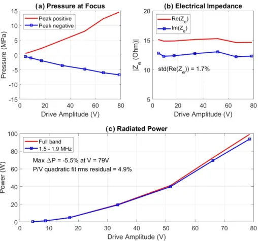
characterization. . . 42 2.4 Comparison of electrically estimated and acoustically measured power

outputs of the H-102 (SN: B-022) transducer. . . 47 2.5 Comparison of electrically estimated and acoustically measured power

outputs of the H-107 (SN: 031) transducer. . . 48 2.6 Validation of the small-signal electrical impedance measurement re-

sults to higher driver voltages (resulting in higher pressures and powers). 50 3.1 Components of the cumulative correlation signal. . . 57 3.2 Method for calculating the map of time constants via exponential

curve fitting to autocorrelation functions of pixelwise temporal RF signal changes. . . 59

(9)

3.3 Spatial map of time constants calculated from fitted exponential curves. 61 3.4 A (typical) B-mode (brightness-mode) US image from the image se-

quence (as reference for Fig. 3.3). . . 61 3.5 Example of the results of decorrelation analysis for pixels imaged in

the central ventral region of the mouse. . . 62 3.6 Long-term tissue effects. . . 63 4.1 Schematic illustrating the concept of conventional DABAS methods. . 71 4.2 Schematic illustrating the concept of the proposed rt-DABAS method. 73 4.3 Example of position estimation output for showing the concepts of

bias and ripple errors. . . 74 4.4 Excitation signal used for simulations. . . 79 4.5 Schematic of the experimental setup of phantom experiments. . . 80 4.6 Simulated B-mode images of homogeneous phantoms of 0.2, 1, 5 and

10 scatterers/resolution cell densities. . . 85 4.7 Simulated B-mode images of 1, 11 and 31 scatterers respectively

placed around transducer focus with a uniform axial spacing of 1 mm. 86 4.8 B-mode ultrasound image made of a 3% agar – 4% graphite homoge-

neous phantom. . . 86 4.9 Calibration curves calculated from simulated data of homogeneous

phantoms with 0.2, 1, 5 and 10 scatterers / resolution cell densities. . 87 4.10 Calibration curves calculated from simulated image data of a homoge-

neous phantom without noise and with additional (Gaussian random distribution) noise according to 20 dB, 15 dB, 10 dB, 5 dB, 0 dB and

−5 dB SNR. . . 88 4.11 Calibration curves calculated from simulated image data of 1, 11 and

31 scatterers (placed axially around transducer focus with a uniform 1 mm distance) compared with the calibration curve calculated from the simulated image of a FDS homogeneous phantom. . . 90 4.12 Calibration curve from experimental image data. . . 91

(10)

4.13 Position estimation errors for simulated data of a FDS homogeneous phantom using fixed and adaptive calibration curves. . . 94 4.14 Position estimation errors for experimental data of a homogeneous

agar-graphite phantom using fixed and adaptive calibration curves. . 95 4.15 In vivo ultrasound images of a melanoma on a human sole. . . 98 4.16 Examples showing the performance of the preprocessing method de-

veloped for automated axial correction of data frame sequences. . . . 99 5.1 Components of the portable, cost-effective skin imaging ultrasound

device prototype. . . 106 5.2 Comparison of ultrasound images of a basal cell carcinoma generated

by a commercially available reference device and by the portable device.110 5.3 Comparison of corresponding ultrasound images obtained with a com-

mercial reference device and with the proposed portable skin imaging device and of photographs taken of the slices used in histological examination of the same lesions (melanoma, keratosis seborrhoica and basalioma). . . 111

(11)

List of Tables

4.1 Ranges of position estimation errors within the 150–350 µm range of image grid step sizes for a simulated FDS phantom using fixed and adaptive calibration curves. . . 96 4.2 Ranges of position estimation errors within the 150–350 µm range of

image grid step sizes for the agar-graphite phantom experiment using fixed and adaptive calibration curves. . . 96 4.3 Scan conversion algorithm performance for in vivo (human skin tis-

sue) data based on 20 lesion dimensions. . . 97

(12)

List of Symbols

A amplitude

A_T area (of transducer active element surface) a air (material symbol)

α acceptance criterion (rt-DABAS) c speed of sound

D aperture of ultrasound transducer d distance

∆ difference

∆y image grid step size e_b bias error

e_r ripple error

threshold for acceptance criterion (rt-DABAS) F focal length

F_i incoming data frames (DABAS) F[ ] Fourier transform

f frequency

f(t) temporal function f⁰(t) time derivative of f(t) G_{f ocal} focal gain

g glycerine (material symbol)

H_r focal plane beam pattern (hydrophone measurement) h hydrophone spatiotemporal response

(13)

I electric current

I_k image frame (DABAS) J window size (rt-DABAS) λ wavelength

M_h hydrophone sensitivity

m material (general material symbol) N number of samples

N_d near-field distance

n number of samples (data points) in a signal or number of frames in an image

P power

P_a acoustic output power

P_deg power required to raise the temperature of tissue by 1^◦C P_t total power consumption

p pressure

p_r peak rarefaction pressure ρ₀ density of a medium ρ(d) calibration curve

ρ_xy Pearson correlation coefficient σ signal-to-noise ratio

T_surf transducer surface temperature t time

τ time constant (of an exponential function) V voltage

V_rms root mean squared voltage v velocity (scanning speed) w water (material symbol) w(j) weights (rt-DABAS)

x vector of impedance parameters used in linear system of equations for two-port model parameter estimation

(14)

y positions

y_d desired positions y_t true positions

Z electrical impedance

Z₀ characteristic acoustic impedance of a medium Z_L characteristic acoustic impedance of a load medium

z axial distance from ultrasound transducer surface

(15)

List of Abbreviations

1-D: One-dimensional 2-D: Two-dimensional 3-D: Three-dimensional A-line: Amplitude-line A/D: Analogue-to-digital

ABCD: Asymmetry, Border irregularity, Color variegation, Diameter >6 mm ABCDE: ABCD, Evolving

ATP: Adenosine triphosphate B-mode: Brightness-mode BCC: Basal cell carcinoma

CLSM: Confocal laser scanning microscopy

CMUT: Capacitive micromachined ultrasonic transducers DABAS: Data-based scanning

DECUS: Decorrelation ultrasound DOF: Depth of field

ESWL: Extracorporeal shock wave lithotripsy FDS: Fully developed speckle

FNAC: Fine needle aspiration cytology FWHM: Full width at half maximum HIFU: High-intensity focused ultrasound

IEC: International Electrotechnical Commission KLM model: Krimholtz-Leedom-Matthaei model MI: Mechanical index

MRI: Magnetic resonance imaging

(16)

mRNA: Messenger ribonucleic acid NDT: Non-destructive testing

OCT: Optical coherence tomography PLA: polylactic acid

PRF: Pulse repetition frequency

RF: Radiofrequency (RF signal: raw ultrasound signal) RFB: Radiation force balance

RMS: root mean square

RMSE: root-mean-square-error

rt-DABAS: Real-time data-based scanning SCC: Spinal cell carcinoma

SLNB: Sentinel lymph node biopsy SNR: Signal to noise ratio

TGC: Time-gain compensation TI: Thermal index

US: Ultrasound

USD: United States dollar USI: Ultrasound imaging UV: Ultraviolet

(17)

Chapter 1 Introduction

1.1 Motivation and overview

It is impressive to realize the diversity of ultrasound waves themselves and of the application potentials of ultrasound technology, from imaging (lifeless materials [6]

as well as living tissues [7]) to therapy [8], from simple distance measurements to velocimetry and elastography [9], from conventional ultrasound signal generation and recording to optoacoustic imaging [10], from low energy data transfer [11] to security applications [12], etc. It is also exciting to realize the trends towards making the ultrasound devices more and more portable (due to technological advances and creative ideas) [13] and user-friendly (with the aid of artificial intelligence and other increasingly sophisticated methods) [14]. Finally, it is interesting how simple ideas can lead to significantly beneficial results in this field if the necessary technological background is provided.

The work presented in this thesis focuses on small but forward slices of this exciting, diverse world. The focus is basically on changes in ultrasound signals.

Changes are investigated in various ways, as described in Section 1.1.1 below. The motivation of this work was not only the beauty an excitement of research but also taking advantage of the findings for wide-spread point-of-care and cost-effective use and calibration of ultrasound devices.

(18)

1.1.1 Summary

The thesis focuses on three topics related to ultrasound technology. Regarding ultrasound imaging, novel correlation methods – exploiting signal changes – are presented and discussed: one taking advantage of temporal (Chapter 3) and another of spatial information (Chapter 4), in sequences of ultrasound signals. Both methods lead to applications in diagnostic ultrasound imaging, primarily. In particular, a portable and cost-effective diagnostic ultrasound device specified for skin imaging is presented in Chapter 5, taking advantage of the spatial correlation method presented in Chapter 4.

An additional topic is the presentation and discussion of an impedance-measurements- based method – exploiting impedance changes – for ultrasound transducer characterization (Chapter 2), as a novel approach in this field. Since this topic is related to the technical background of the application of ultrasound, the topic precedes the thesis chapters discussing the novel correlation methods in imaging. Characterizing the acoustic output of ultrasound transducers in a fast, practicable and cost-effective manner can be of great advantage in several fields including diagnostic, therapeutic and non-medical applications of ultrasound technology. In particular, it is applicable for determining safety of the skin-diagnostic device presented in Chapter 5.

1.1.2 Overview of current thesis

Following this overview, Chapter 1 introduces both the physical background of ultrasound imaging and the diagnostic area of application – in particular dermatological ultrasound for skin cancer imaging – which is the practical motivation of the most prominent part of this work. Ultrasound imaging background is discussed in terms of ultrasound imaging physics and of systems for ultrasound imaging (see Section 1.2).

A separate section (Section 1.3) briefly introduces the bioeffects of ultrasound.

This topic is of particular relevance to the results presented in Chapter 2. It is followed by another brief section presenting the mathematical basics of correlation calculation (Section 1.4) which will be used in Chapters 3 and 4.

As mentioned above, the primary motivation for the application of the proposed

(19)

methods is skin cancer diagnosis. The introduction of skin cancer and remarks on the importance of its early detection is followed by a short review of approaches for skin cancer diagnosis (see Section 1.5). The relevance of ultrasound imaging is highlighted among the approaches.

In Chapter 2, acoustic output characterization of ultrasound transducers is discussed, presenting the theory and validation of a novel method based on impedance measurements.

As shown in the subsequent chapters, data correlation was investigated in two aspects: temporal correlation and spatial correlation, leading to two novel methods with different applications.

In the method discussed in Chapter 3, temporal correlation is used for detecting the extent of dynamic changes at certain spatial points (pixels) in a series of ultrasound images acquired at the same spatial location. The method is validated on the application of showing the dynamics of post-mortem tissue effects.

Spatial correlation was also used for distance estimation of 1-D ultrasound data leading to the application of freehand manual scan conversion (without using position sensors) in 2-D imaging. In Chapter 4, the theory behind the proposed real- time data-based scan conversion method is presented, followed by validation of the algorithm. The validation was performed on simulations and experiments using homogeneous agar-graphite phantoms. Application and clinical validation of the proposed data-based scan conversion method is presented in Chapter 5. Clinical experiments were performed using a custom device, which was built for cost-effective in-vivohuman skin imaging for skin cancer diagnosis, utilizing the presented imaging method.

Chapter 6 summarizes the thesis points concluded from the work presented in the previous chapters (Chapters 2–5).

(20)

1.2 Introduction to ultrasound imaging

1.2.1 Ultrasound imaging physics

Ultrasound

Ultrasound is widely used in clinical investigations nowadays (being used in around 20–25% of clinical imaging examinations [7]). It has several and diverse application fields including therapeutic applications, industrial ones (like non-destructive testing) and navigation. Hereinafter, the topics of this thesis focus on applications in imaging with clinical motivation, therefore the introductory sections are written accordingly.

Ultrasound imaging uses high frequency mechanical waves for localizing and characterizing objects or edges of objects from which these waves reflect, inside media in which the waves are able to propagate. By definition, ultrasound can be any mechanical wave with a frequency above 20 kHz [15]. However, for imaging, significantly higher frequencies are tipically used (∼MHz range for acceptable resolution in medical imaging) [16, 9].

There are several types of sound waves (propagating mechanical vibrations) being suitable for different applications (eg. shear waves, longitudinal waves, surface waves, Lamb waves) [17]. In the methods discussed in this thesis, hereinafter, the sound waves being applied arelongitudinal ultrasound waves.

Ultrasound transducers

Mechanical waves can be generated and measured by using some type oftransducer: a device that converts variations in a physical quantity (such as pressure in the case of longitudinal ultrasound waves) into an electrical signal, or vice versa [17]. An ultrasound transducer can convert an electrical signal into a pressure wave generated via mechanical vibrations. The same transducer is capable of measuring pressure variations induced by incoming ultrasound waves, via mechanical vibrations, and converting them into electrical signals.

(21)

Pulse-echo method

Ultrasound technology is widely used for a variety of applications utilizing different properties and features of these mechanical waves. For ultrasound imaging, the most commonly used technique is the pulse-echo method.

Figure 1.1: Schematic of the pulse-echo method. In transmit, the transducer converts the excitation pulse into mechanical wave packet which propagates in the direction designated by the transducer. The wave packet gets scattered on inhomogeneities of the propagation media. The backscattered waves are converted into a temporal electrical signal (‘A-line’) by the receiving transducer.

In pulse-echo mode, a longitudinal ultrasound pressure wave packet (pulse) is sent from a transducer (this step is called thetransmit). As the wave packet propagates through the media of examination, it gets scattered on inhomogeneities of the media (Fig. 1.1). Ultrasoundscatterers – the above-mentioned inhomogeneities

(22)

– present as variations in density and compressibility [7, 9, 15]. The term backscat- tered wave stands for scattered wave packets that propagate towards the receiving transducer (being equal to the transmit transducer, in the case where the term

“backscattering” is used) [7, 16]. During the step of receive, backscattered wave packets (echoes, in response to the transmitted pulse) are received by the receiving transducer (being usually identical to the transmitting transducer) which converts the pressure variations of the incoming wave packets into a temporal electrical signal (as noticed above) [17]. Basically, two quantities are being measured together in pulse-echo receive: amplitude of the received signal and time of signal arrival in reference to the time of transmit. In this way, the receiving transducer collects information about scatterers with different scattering strength (occurring in amplitude measurements of scattered waves) in a certain direction – along a 1-D line (Fig. 1.1).

Such information of temporal amplitude changes (in a 1-D electrical signal, referring to pressure amplitude changes induced by 3-D backscattered wave packets reaching the receiving transducer surface) is called an A-line (or A-scan) [9].

Assuming that the propagation speed of ultrasound is known in the media of examination, a temporal signal (in t) can be converted into a spatial signal (in z), using the equation:

z =ct/2, (1.1)

wherec is the assumed propagation speed of sound in the medium of examination.

The division by 2 takes into account that the wave packet traveled forth and back during the time measured between transmit and receive [9].

Pulse-echo data processing

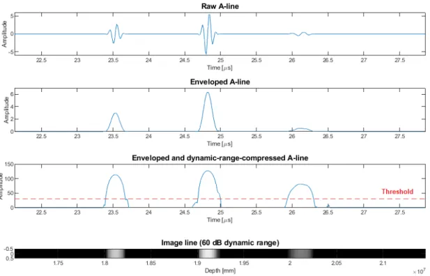
Applying the technique of envelope detection on the biphasic raw A-line signals results in a monophasic 1-D signal which represents scatterers (with their scattering strength) and their spatial positions, along the line. Scattering strength can be de- duced from the relevant peak amplitude (of a backscattered wave packet) occurring in the A-line, while taking into account the attenuation of the media in which the sound waves propagated forth and back, the acoustical shading effect (coming from the fact that scattering commutatively degrades the amplitude of the wave passing

(23)

Figure 1.2: Basic steps of signal processing for ultrasound A-lines (presented for the example shown in Fig. 1.1). Raw biphasic A-line signal; Enveloped A-line; dynamic- range-compressed A-line with threshold for noise rejection in display; B-mode display of A-line.

on) and some interference of the backscattered waves and their harmonics [18].

The enveloped A-line signals can easily be represented and displayed as a 1-D series of image pixels in which color (or intensity in the case of a gray-scale representation) of a pixel corresponds to the enveloped amplitude of the backscattered signal (and thus to the strength of scattering in that certain point in space, which point is calculated from time and sound speed due to Eq. (1.1)). Such representation is the basis of the so-calledB-mode (or brightness-mode) ultrasound images (Fig. 1.2).

For better interpretability of the received signals of varying amplitude peaks – for displaying a wider range of information – A-lines are usually displayed after applying dynamic range compression (usually done via logarithmic amplification) [9].

A threshold for data display is also usually applied for rejecting noise (Fig. 1.2).

(24)

Scanning

In order to get a 2-D image, several A-line envelopes (in pixel series representation) should be put beside each other considering their relative spatial dispositions. 3-D images are usually created in a similar way from 2-D images (in this case, 2-D images are the blocks being put side by side with proper spatial positioning) [19].

As discussed above, ultrasound images generated using the pulse-echo technique are generally obtained from 1-D lines of ultrasonic signals. 2-D or 3-D ultrasound imaging requires a sequence of lower dimensional data with known relative positions to be geometrically placed alongside each other. This process is termed scan conversion [9]. Scan conversion is performed on data acquired in multiple spatial directions (one being the direction of the pulse-echo measurement and at least one distinct spatial direction), during the process of scanning.

Regarding ultrasound scanning, three directions are discerned: axial, lateral and elevational. Axial direction is the term for the primary direction in which the pulse and echoes propagate. Lateral direction is perpendicular to the axial direction and is usually the direction in which scanning is performed for obtaining a 2-D image.

Elevational direction is perpendicular to both of the former ones, usually indicating the dimension pointing out from a 2-D image plane.

Physical characteristics of an ultrasound beam for imaging

Following a short introduction of the concept of ultrasound beams, the most important parameters and phenomena are shortly discussed here in relation to ultrasound imaging, such as resolution (in different directions), causes of attenuation, sound speed, acoustic impedance and pulse repetition frequency.

Spatial resolution of an ultrasound image as well as penetration for imaging is defined by the characteristics of the ultrasound beams formed and measured in the pulse-echo method. Theoretically two beams – transmit beam and receive beam – can be considered [9]. The transmit beam implies the changes introduced by the transmitted pulse into the pressure field in front of the transducer. The receive beam is (not a physical beam, but) a concept describing the parts of the pressure field which contribute to the signals being able to be received by the receiving

(25)

transducer. For a single-element transducer (or for an array transducer not using dynamic focusing, nor dynamic apodization) that is being applied for both transmit and receive, the two beams can be treated as being identical. (The above-mentioned dynamic focusingand dynamic apodization are methods being used for changing the receive beam characteristics dynamically. Since these methods are applicable for multi-element – array – transducers only, these topics are out from the scope of this thesis.)

Spatial resolution of ultrasound images is specified by the length of the transmitted wave packet (axial resolution), by the focusing characteristics of the beam (lateral and elevational resolution) and by attenuation characteristics of the media of examination (since attenuation modifies the frequency band of the propagating wave, and in this way, it also modifies the resolution in all three directions [9]). Wave packet length is a function of the frequency band of the transmitted pulse and of the sound propagation speedinside the media of examination. For a certain sound speed, the greater the central frequency or the narrower the frequency band is, the better the resolution. However,penetration depth follows the opposite trend, due to the nature of Rayleigh scattering (higher frequency waves – with shorter wavelengths (close to the order of scatterer dimensions) – are being strongly scattered, thus the lower the frequency, waves – having a longer wavelength – penetrate deeper) [17].

In this way, acoustic attenuation acts like a low-pass filter on the sound waves.

Attenuation of ultrasound waves can be caused by different physical phenomena: scattering (as described above), diffraction and absorption (kinetic energy of the wave transforming into thermal energy of the propagation media) [18]. Reflec- tion is a special case of scattering: causing scattered waves propagating back in the direction which they came from.

Propagation speed of sound (or sound velocity) is determined by thedensity and theelastic modulus (related to compressibility) of the medium. Although, to be accurate,group speed andphase speedof sound waves should be treated separately, it is commonly adopted in medical ultrasonic applications to describe sound speed with a single, amplitude-independent value that can be measured for any specific medium, since velocity dispersion does not appear to be significant in the frequency ranges and

(26)

precision of these applications [7]. As already mentioned, sound speed is material- specific (tissue-specific, accordingly), and it is also affected by temperature, state (solid/liquid/gas) and pressure of the material [7]. These conditions of the media of interest therefore have to be taken into account when performing the conversion from time to distance on pulse-echo image data.

It is important to introduce the concept of theacoustic impedance, as a useful descriptive of media with different acoustical properties. The acoustic impedance relatespressure and particle velocity. For locally plane waves (in inviscid medium), the characteristic acoustic impedance Z₀ is specified by the density of the medium (ρ₀) and the sound speed in it (c₀): Z = Z0 = ρ0c0 [17, 7]. The characteristic acoustic impedance of different media are very useful descriptors when considering propagation of sound waves in different media. The higher the difference in this impedance value is for two media, the stronger the reflection is from the boundary between them. It also follows that wave propagation in media with equal characteristic acoustic impedance suffers no reflection at all. It is easy to see that knowledge of characteristic acoustic impedances is very useful when describing or predicting wave propagation through different media. (These values and their differences should be considered in particular when imaging biological tissue.) Acoustic impedance is usually expressed in units of Rayleighs (Rayl; 1Rayl = 1P a·s/m) [17]. Regarding fluids and solids used in ultrasound technology or examined in biological samples, typical values are in the range of M Rayl (10⁶Rayl). It is important to note here that soft tissues have similar characteristic acoustic impedances due to their high water content [9].

Focusing of ultrasound beams has already been mentioned above when discussing spatial resolution of ultrasound images. A natural focus arises for every ultrasound transducer, due to their finite aperture. The natural focus is determined by thenear-field distance N_d of the transducer with a certain apertureD, transmitting or receiving waves of frequency f in a medium with sound speedc [18]:

N_d= D²f 4c = D²

4λ . (1.2)

There is a simple geometrical reason behind this, namely that spherical wavelets

(27)

originating from different points of the aperture (and forming the wavefront) form an interference pattern of constructive and destructive interferences within the near- field distance [9]. However, there exists a distance from which the interference can only be constructive: this boundary is called the near-field distance, the value of which geometrically comes from the size of the transducer aperture (D) and from the wavelength (λ) as shown above. Since in the far field (in distances larger than the near-field distance) the pressure amplitude of the spreading wave degrades gradually, a natural focus occurs at the near-field distance of the transducer, being specific for the frequency of its waves.

There are further techniques for focusing an ultrasound beam, in a more plannable manner. Focusing can be achieved using specific transducer geometry, using acous- tic lenses or by applying relative phasing in the case of array transducers [7, 9].

Transducers can be manufactured in a way to have a geometry which focuses the ultrasound beam emitted (and also focuses at the same region for receiving beams).

In the cases of concave, spherically curved transducer geometries, focal length is defined by their radius of curvature. Acoustic lenses can be put in front of the transducer using a material in which sound speed differs from that of the loading medium (medium examined). Here, focusing characteristics can be designed by the shape of the lens and the ratio of lens and loading medium sound speed [7]. In the cases of array transducers, with the ability of beamforming by relative phasing of elements of the array, focusing can be achieved electronically, in a programmable way, with the great advantage of being able to change the focus between transmission and receive and even to change the focus dynamically (e.g. during receive).

Important measures of the focusing characteristics are the focal gain factor, full width at half maximum, depth of field and focal length of the sound beam [9]. Focal length (F) is defined by the distance of the focus from the surface of the transducer.

Focal gain quantifies the pressure gain achieved at the focus in relation to the pressure amplitude at the transducer surface. In general, focal gain is defined by the aperture (D), area (A_T), focal length (F) of the transducer and by the wavelength (λ) of its wave [9]:

G_{f ocal}= DA_T

λF . (1.3)

(28)

In the cases of unfocused transducers,G_{f ocal}= 2 gives a good estimate of the natural focus.

In order to characterize the focal region of the beam, beam diameter of at least

−6 dB intensity of that of the peak is given by the full width at half maximum (FWHM)value. On the other hand, the focal zone in the axial direction is given by thedepth of field (DOF) value which, in general, is also calculated for −6 dB of the peak intensity [9, 18].

In pulse-echo imaging, subsequent pulses are sent repetitively in order to acquire multiple data frames in time. This can be used either for acquiring data of temporal changes (at a constant spatial location) or for performing scanning (by physically moving the transducer and acquiring data in multiple dimensions). The parameter defining how often pulses are sent in an ultrasound transmit transducer is called the pulse repetition frequency (PRF) [9]. The frame rate of an ultrasound imaging system using a single-element transducer is equal to the PRF. For multi- element transducers, the frame rate is determined also by the number of image lines and – in some applications using multiple focal zones for each line – by the number of transmissions required for each line, together with the number of image lines [17].

In contemporary ultrasound imaging systems, a PRF in the order of hundreds of Hz or several kHz is applied usually.

1.2.2 Ultrasound imaging systems

The basic components of ultrasound imaging systems are shortly discussed hereinafter. An electrical signal is generated in the waveform generator, which signal drives the transmit transducer. The transducer converts the drive signal into mechanical vibrations due to the desired waveform. If the same transducer is used for transmit and receive, a transmit / receive switch (built into the path between the waveform generator and the transducer) accomplishes the task to switch for receiving and forwarding signals from the transducer to the signal processing network and to switch back for driving the transducer for a new pulse transmission – after a certain period of time determined by the PRF. The received signals – acoustic waves picked up and converted into an analogous electrical signal by the transducer – are digitized

(29)

by an analogue-to-digital (A/D) converter for further signal processing. The basic steps of signal processing are envelope detection, dynamic range compression and scan conversion (image formation), as described previously.

Regarding physical realization of systems for ultrasound imaging, hereinafter two topics – ultrasound transducers and scanning – are discussed as being important for the scope of the current thesis.

Ultrasound transducers

There are several physical phenomena which can be used for conversion between electrical and mechanical vibrations. Electromagnetic (cf. dynamic microphones), electrostatic (cf. condenser microphone, CMUT – capacitive micromachined ultrasonic transducers), magnetostrictive, electric spark (cf. ESWL – extracorporeal shock wave lithotripsy – transducers), radiant energy (cf. opto-acoustics) and piezoelectric effects are all transduction mechanisms which are proven to being applicable in ultrasound transducer technology [17]. Nevertheless, the most commonly used transduction mechanism of the above, currently, is the piezoelectric effect, being used for both transmission and receive [17].

The piezoelectric effect can manifest in crystals having crystal structure without central symmetry [17]. Mechanical strain applied on these crystals results in electrical polarization (due to the electrically asymmetric crystal structure) – this phenomenon is termed the direct piezoelectric effect. On the other hand, inverse piezoelectric effect also manifests in these crystals, meaning that applying voltage on (opposite) sides results in mechanical deformation of the crystal. The inverse piezoelectric effect is applied in transmit and the direct effect is applied in receive mode of piezoelectric ultrasound transducers.

In physical realization, a typical piezoelectric ultrasound transducer consists of the (relatively flat) piezoelectric crystal (also called the active element) with electrodes on both (front and back) sides connected to a connector (of some electrical connector standard), put inside an external housing encasing thebackingmaterial on one side (the back side) of the crystal [18] (Fig. 1.3). The material used as backing

(30)

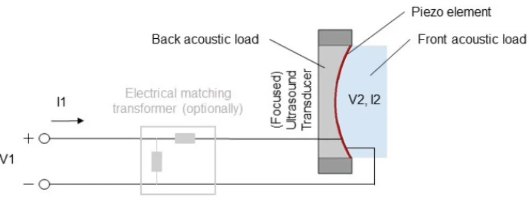
Figure 1.3: Schematic showing the main components of a piezoelectric (focused) transducer.

load is usually highly attenuative in order to absorb energy going into the backing direction and is chosen with respect of the intended use of the transducer. Pulse characteristics such as waveform duration and signal amplitude can be tuned via selection of the backing material regarding its characteristic acoustic impedance in relation to that of the crystal itself. With larger mismatch in characteristic acoustic impedances of the two materials, longer waveform is generated with higher signal amplitude (due to the stronger reflections from the crystal-backing interface) [18].

Choosing a backing load with a better match in acoustic impedance results in lower amplitude but more damped waves emitted into the material of interest, providing a better resolution for pulse-echo imaging. Choice of the former case (larger mismatch in acoustic impedance) is usually more appropriate when fabricating transducers for therapeutic applications while the latter case is beneficial for diagnostic ultrasound transducers. Central – resonance – frequency of the transducer is defined by the thickness of the piezoelectric crystal, while bandwidth of its pulse is defined by the backing material as described above. In order to reduce reflections from bound- aries between the crystal and a medium with mismatching characteristic acoustic impedance, one or morematching layer(s) can be applied on the relevant surface of the crystal, consisting of a material with characteristic acoustic impedance value being in between those of the crystal and the medium. A commonly used arrangement is having a matching layer of thicknessλ/4 on the front surface of the active element crystal (of lengthλ/2), in order to achieve a larger amplitude (and coherent) signal transmission into the front medium [18].

(31)

Severalequivalent electric circuit modelsexist for piezoelectric ultrasound transducers. A widely used and commonly accepted model is the so-called “KLM model”

[20]. Electrical and mechanical parts of the circuit are being distinguished in this model. An acoustic transmission line with two ports accounts for the transducer converting electrical into mechanical energy on both front and back surfaces. A network of frequency-dependent components connects the acoustic transmission line to a third port accounting for connection with the electrodes. Equivalent circuit models are very useful for predicting or simulating the performance of transducers.

Performance criteria – such as efficiency, dynamic range and pulse characteristics (bandwidth, pulse duration) – can be optimized by using these models. In the KLM model, the above characteristics can be simulated (and optimized) for physical properties of the transducer material (physical dimensions, acoustic impedance, sound velocity and coupling factor of the piezoelectric ceramic), of the possible matching layer(s) (physical dimensions, acoustic impedance), of the backing load and front load (acoustic impedance) and of the electrical tuning of the transducer [21]. Mod- els like the KLM model have played an important role in designing piezoelectric ultrasound transducers and have also been further developed in order to become able to account for various real-life phenomena such as mechanical, dielectric and piezoelectric losses of energy [22].

Scanning

As introduced in Section 1.2, pulse-echo ultrasound images are technically built up from 1-D data lines. The process used for dimension incrementation is generally termed scanning. Currently used physical realizations of scanning can be summa- rized in the following groups [19]:

1) Electronic scanning, 2) Mechanical scanning,

3) Free-hand scanning with position sensors, 4) Free-hand scanning without position sensors.

Given the importance of this topic regarding the current thesis, the above approaches of scanning are discussed in a separate subsection, as follows.

(32)

1.2.3 Scanning methods for ultrasound imaging

The following is a review of different, currently available scanning methods for ultrasound imaging. For further information, the reader is referred to [19, 4].

Electronic scanning

Image dimension can be incremented without any physical movement when using a multi-element transducer. In the case of a ‘linear array transducer’, multiple transducer elements are arranged along a line (Fig. 1.4). The beam of these multi- element transducers can be focused in several directions along a plane. In a similar way, the focus of the transducer can be varied by using different delay profiles (delay being a function of transducer element position) before signal summation in the receive mode. In this way, multiple axial scans (A-lines) can be collected in the lateral direction.

Figure 1.4: Schematic illustrating the concept of electronic scanning using a (multi- element) linear array transducer.

Considering the case of transducer elements being placed on a 2-D plane, 3-D images can be scanned electronically in a similar way (by varying the delay profile on the 2-D array of elements).

The great advantage of electronic scanning is that it is a real-time method for multidimensional scanning with precisely known information of the spacing of scans and without any physical movement needed. However, array transducers require

(33)

complex electronics and multiple transducer elements, hence they are not cost- effective [19].

Mechanical scanning

A widely used approach for incrementing image dimension is to move the transducer physically in a direction in which dimension incrementation is desired. However, in order to avoid distortion, it is necessary to know the relative location and orientation of the single (lower-dimensional) scans. Mechanical scanning techniques use a motorized mechanical apparatus to physically move a transducer with precisely known location and orientation [19].

Linear mechanical scanners move the transducer along a line in order to acquire a series of parallel images. Besides its spatial precision, this method has the advantage of collecting images with equal spacing, thus a smooth resolution can be obtained.

As a disadvantage, a mechanical scanner apparatus is a bulky device, hence it is not very convenient to use [19].

Another commonly used approach is to tilt the transducer (Fig. 1.5), obtaining fan-like images with equal angular spacing [19]. Tilt scanners are convenient to use and not bulky (as compared to the linear scanner devices), but have the disadvantage of uneven resolution in different depths [19].

Figure 1.5: Schematic illustrating the concept of mechanical scanning using tilting motion of a single-element transducer.

A third possible technique is rotational scanning in the case of 3-D imaging.

(34)

In this method, rotation is performed along the axial axis. Rotational scanning has similar advantages and disadvantages to tilt scanning, having the additional disadvantages of an even more complex resolution distribution and the risk of having artifacts based on possible physical displacement of the axis of rotation [19].

In summary, mechanical scanning has the advantage of precise position determination and fast reconstruction time [19], but also has the general disadvantages of potential failure of the motorized system and of physical limitations of the area (or volume) in which scanning can be performed.

Free-hand scanning with position sensors

In order to get rid of the above disadvantages and limitations, free-hand scanning can be used, providing more convenience and freedom. Determination of the relative locations and orientations of single scans is achieved in most of the cases by the usage of position sensors (Fig. 1.6). There are several types of sensors successfully combined with ultrasound transducers.

Figure 1.6: Schematic illustrating the concept of freehand scanning using a single- element transducer combined with some type of 3-D position sensor.

In the case of using acoustic sensors, (low-frequency ultra)sound is emitted from three separate locations on the transducer casing surface and measured by three microphones (located somewhere near the object of examination). One of the main limitations of this technique is that the line between the transducer and the micro-

(35)

phones should be left free. The other disadvantage is that sound speed varies with humidity in the air [19].

Another approach uses articulated arms (conjoining the transducer with a fixed location). In this case, relative movements are measured by potentiometers located in the joints of the arms. As a limitation, larger flexibility of the arms leads to worse resolution of position sensing. However, by decreasing the length of the arms (in order to reduce flexibility) leads to another disadvantage: a reduced maximum size of scanning area or volume [19].

Probably the most successful position sensors for free-hand scanning are the magnetic sensors. These little sensors provide convenience and freedom. However, the magnetic field distortion of ferrous metals can cause artifacts when using these systems [19].

Free-hand scanning without position sensors

There is an interesting potential for position estimation even without additional sensors or external devices, taking advantage of the “speckle pattern” of ultrasound images (Fig. 1.7). Speckles are common features of ultrasound images. The speckle pattern evolves from interference caused by interaction of the ultrasound field and the scatterers [19]. Although they are commonly treated as artifact, speckle pat- terns may contain important information about the imaging system and the examined medium [23]. Data-based scan conversion makes use of the speckle pattern of ultrasound images. The idea is based on the correlation between two parallel images. If the images are close enough to each other, the speckle pattern causes a high correlation between them. When moving away from a certain line, the calculated correlation value is decreasing even in homogeneous media, again, due to the presence of the speckle pattern. There is a specific dependence between distance and correlation, which can be described by the so-called decorrelation function (in terms of distance).

A great advantage of these methods is that they can be applied on transducers without any hardware modifications [7]. Another important advantage is the lack

(36)

Figure 1.7: Schematic illustrating the concept of freehand scanning without position sensors. In data-based scanning approaches, the relative positions of the A-lines are estimated from speckle correlation (middle), knowing the distance-correlation dependency(right).

of spatial limitations for the area scanned, achieved without the disadvantages, cost and complexity of the above position sensors. On the other hand, calibration is necessary and reliability is usually not enough for distance-based measurements (in the scanning direction) on these images [19, 7].

1.2.4 Data-based scan conversion approaches

In order to perform scan conversion based on correlation, an accurate calibration curve should be obtained. The term calibration curve refers to a function, that describes a one-to-one relation between distance and correlation. Much research focuses on the proper determination of this function. Conventional methods use a nominal decorrelation curve obtained from an (ideal) fully developed speckle (FDS) [24]. The nominal decorrelation curve is stable for a certain transducer [25].

Furthermore, several adaptive algorithms exist [26] that use an ideal phantom for obtaining the nominal decorrelation curve and then use adaptive models to get dynamic decorrelation curves [27]. There are techniques for speckle tracking without FDS using modeling of the raw ultrasound signals generated by speckles [23]. Sev- eral studies perform statistics on the image data in order to get a more suitable calibration curve (based on some statistical features of the examined object and of the signals generated by the imaging system). It has been shown that estima-

(37)

tion of the envelope statistics allows characterization of tissue regularity and thus estimation of the calibration curve [25].

1.3 Biological effects of ultrasound

As the main scope of this thesis is in medical ultrasound diagnostics and furthermore, since one of the novel methods presented and discussed here (in Chapter 2) points towards the application of determining safety parameters of ultrasound equipment in a new way with several advantages, biological effects of ultrasound and their measures are briefly introduced here.

Ultrasound imaging and therapy forms a type of radiation of mechanical wave beam into the media of examination, ie. tissue in the case of biological samples.

Regarding safety, an outstanding biomedical advantage of ultrasound is the lack of ionizing effect of its radiation. For safe use of ultrasound, nevertheless, two aspects – namely the mechanical and thermal effects – should be kept within limits.

Mechanical effectsarise from ultrasound waves introducing pressure variations in the tissue in which they propagate. Thermal effectsarise from tissue absorbing some of the mechanical energy of the sound waves and also from the heat of transducer propagating from the transducer surface in tissue regions being near to it [28].

Standards of the International Electrotechnical Commission (IEC) define the mechanical index (MI) and thermal index (TI) values which should be verified for biomedical ultrasound systems to be within certain limits regarding the application.

As mentioned above, an additional safety measure of transducer temperature rise should also be proved for claiming safety, especially for the cases of having temperature sensitive tissue within about 5 mm from the transducer surface [28].

1.3.1 Mechanical index

Ultrasound, as a pressure wave propagating through tissue, causes compression and rarefaction in successive cycles at specific locations of the tissue. If the peak rarefaction pressure is large enough, bubbles may come to be in the tissue (fluid) [7]. This effect is calledcavitation and is very useful in several therapeutic applications of ul-

(38)

trasound [29] but is to be avoided in numerous fields of the body including arteries (in which arising microbubbles would lead to serious consequences). Therefore, the MI of diagnostic ultrasound machines should be kept within safety limits in which cavitation is theoretically not possible to occur.

MI is defined by the peak rarefaction pressure (p_r) and the frequency (f) of the ultrasound wave as follows:

M I = p_r,0.3

√f . (1.4)

The peak rarefaction pressure becomes the greatest in the focal region of the ultrasound beam. Due to the attenuation of tissue, pressure values “derated” from those measured in pure water are used for the calculations. Attenuation in soft tissue is usually in the range of 0.5–1 dB/MHz/cm. In safety standards, the absorption value of 0.3 dB/MHz/cm is commonly used (for derated pressure p_r,0.3) leading to a worst-case estimation for MI [28].

1.3.2 Thermal index

By calculating TI, the likely maximum temperature rise due to absorption can be estimated in the tissue [28]. TI is defined as the ratio of the acoustic output power (P_a) of the transducer and the power (P_deg) required to raise the temperature of the tissue by 1 ^◦C [28]:

T I = P_a Pdeg

. (1.5)

Since the presence of bone has a significant influence on the ultrasound-based temperature rise of tissue, different formulae are defined in standards for calculating TI regarding the presence and relative position of bone in the ultrasound beam [28].

1.3.3 Transducer surface temperature

In addition to the thermal effect due to absorption of the sound waves, temperature rise of the transducer should also be considered in superficial tissue being close enough (within about 5 mm) to the transducer surface. Transducer temperature

(39)

rise comes from electrical energy dissipation (of the transducer and of the processing electronics behind) [28]. Limits for transducer surface temperature Tsurf are also defined in safety standards (for different load media).

The above safety indices used for quantifying the biological effects of ultrasound can be calculated based on pressure, power or intensity and temperature measurements. Pressure measurements are usually performed by using a hydrophone measurement system. Intensity can be calculated from pressure. Power measurements are usually done using a radiation force balance (RFB) or calculated from hydrophone measurements. Temperature can be measured using an infrared cam- era (in air) or thermocouples (placed in tissue) [28]. M I and T I values should be indicated to the user of any ultrasound device for which each of these values may exceed the value of 1. Limits forTsurf are 50^◦C in air and 43^◦C in tissue, according to international standards, which means that a 33 ^◦C human skin is permitted to be heated up by about 10^◦C [28].

1.4 The correlation coefficient

In a significant part of this thesis, novel methods utilizing (temporal or spatial) correlation of ultrasound imaging data are presented (as already introduced in Sec- tion 1.1.2). Therefore, a brief introduction of the mathematical basics of correlation calculation is presented here.

The correlation coefficient quantitatively describes a statistical relationship between two variables with a single number. The most commonly used measure of correlation is the Pearson correlation coefficient which measures the linear relationship between two variables regarding strength and direction of the relationship.

The Pearson correlation coefficient is calculated for a pair of variables via divid- ing the covariance of the two variables by the product of their individual standard deviations. For paired data of samples x and y (of equal sample size n):

(x₁, y₁),(x₂, y₂), ...,(x_n, y_n), the Pearson correlation coefficient ρ_xy can be calculated

(40)

from the formula:

ρ_xy =

Pn

i=1(x_i−x)(y_i−y)

qPn

i=1(x_i−x)²^q^Pⁿ_i=1(y_i−y)²

, (1.6)

where x and y denote the mean of samples x and y, respectively, calculated as x= 1/n^Pⁿ_i=1x_i.

1.5 A review of skin cancer diagnostics

1.5.1 Introduction

The motivation behind some of the research that have lead to the results presented in this thesis is an important disease to be treated, of a significant organ of the human body [30]. Skin cancer is one of the most frequent types of cancer in the developed world [31, 32, 33, 34]. Melanoma malignum, a type of skin cancer is responsible for the vast majority of all skin cancer deaths [35]. Fortunately, this type of lesion can be treated safely via surgical excision, but only in its early stage.

Therefore, early and accurate melanoma diagnosis is a crucial problem to be solved in this area [35, 36]. Following an introduction to skin cancer facts, to the structure of the human skin and to some relevant skin cancer types, a review is presented here of relevant invasive and non-invasive diagnostic methods currently used or being under investigation. Potentials in ultrasound-based skin cancer diagnosis are presented in a separate section, showing the versatility of this non-invasive approach for examination purposes.

1.5.2 Background

Skin cancer is reported to be the most common type of cancer in the United Sates [31]

and the third most frequent cancer in Hungary [32]. It is very frequent in many other countries as well (being especially frequent in the Scandinavian countries within Europe) and is extremely frequent in the population of Australia [33]. The lifetime risk for developing skin cancer is around 20% for an average American person [34].

These facts along with other statistical data represent the importance of dealing with these types of cancer.

(41)

The most common skin cancer type is basal cell carcinoma (basalioma), which is a relatively benign cancer as it rarely metastasizes [37]. Melanoma malignum (a type of skin cancer) – the proportion of which is about 1% among all skin cancers [38] – accounts for the majority, 65% of all skin cancer related deaths [35]. As with malignant tumors in general, early detection and treatment of melanoma plays a crucial role in the prognosis and survival of the disease [35, 36]. Earlier detection and treatment (the primary treatment being surgical excision) leads to less morbidity and mortality and even to a decreased cost of therapy [35].

In summary, prevention, early detection (via appropriate diagnosis), adequate treatment and sufficient follow-up of skin cancer diseases is an important healthcare problem to be developed. As melanoma is extremely dangerous compared to most other skin cancer types of less morbidity and far less risk, differential diagnosis (aiming to recognize skin cancer type and to distinguish it from other types) plays a crucial role in skin cancer examination and treatment.

The following review gives insight into the skin diseases to differentiate in between and into the currently used methods for skin cancer diagnosis – as already mentioned above – highlighting the role of ultrasound-based diagnostics as a promis- ing non-invasive approach to assist early detection of melanoma and other types of skin cancer.

1.5.3 Skin cancer

Structure of the human skin

The skin is the largest organ of the human body (weighting 15–20% of the full body mass) [39]. This organ separates and at the same time connects the body and its environment. One of the primary functions of the skin is protection of the body, including physical protection (against mechanical effects and UV radiation), chemical protection (against acids) and biological protection (contra viruses and bacteria). Further functions include homeostasis (thermoregulation, dehydration prevention), sensory role as a touch probe, secretion (of certain chemicals), nutrient storage and insulation (subcutaneous fat tissue) [39]. The skin is composed of three

(42)

primary layers: epidermis, dermis and subcutis.

Theepidermisis the uppermost layer of the skin, generally being less than 1 mm thick (75–600µm, at most 1.4 mm [39]). This layer is composed of 5 sublayers. Cells created at the innermost layers move towards the outermost layer, going through processes of changing shape and composition (keratinization). It is important to note that there are no blood vessels in the epidermis. Several cell types (with different roles) are present in this layer – like keratinocytes, melanocytes, Langerhans cells, Merkel cells, and even lymphocytes.

Among the above cell types, melanocytes are specifically interesting regarding the motivation of melanoma detection. Melanocytes are pigment cells, producing melanosomes that contain melanin – a dye that can absorb UV (ultraviolet) light – and allocating them into neighbouring cells. The number of melanocytes (being around 1% of the total number of skin cells) is almost equal in people regardless of their skin color [40]. However, the amount of melanin (that is responsible for skin, hair and eye color) is greater for people being exposed to stronger UV radiation.

UV radiation causes inflammation in skin being poor in melanin [30].

The (1–2 mm thick) dermis contains blood vessels, nerves, sweet glands and sebaceous glands. The dermis is rich in collagen fibers which provide elasticity to the skin [40].

The innermost skin layer is thesubcutis. It is a loose, connective tissue containing fat storing lipocytes – fat tissue thickness depends on body region (ranging from 0 to 3 cm) [39, 40].

Skin lesions

There are many types of skin cancer and skin lesion. Here, only some of these types are presented below, namely those considered to be the most relevant to the current work.

Nevus (or naevus) is a benign skin lesion containing closely located damaged melanocytes which store melanin (up against healthy melanocytes which produce and then distribute melanin to other cells, and which are distributed relatively homogeneously and far away from each other) [30].

(43)

Nevi can be congenital (presented since birth) or “collected” (which means that they have been developed after birth, at a certain moment in life). Nevi can be located in the junction between the epidermis and dermis (junctional nevus), inside the epidermis and dermis (compound nevus), or deeper in the skin (intradermal nevus).

A nevus may become malignant most probably due to excessive exposure to sunlight (UV radiation), or to physical injury of the nevus. If the nevus becomes changing (its shape, color or size), it can be suspicious of becoming malignant.

Melanoma maligna is the primary malignant skin cancer. Melanoma forms from melanocytes (that is why in many cases it transforms from a nevus – containing spacially concentrated melanocytes). Reasons behind the appearance of this skin disease can be genetical [41], hormonal, virus-induced [42], but in most of the cases it is caused by radiation (primarily UV light). UV radiation, in normal circumstances, is absorbed by melanocytes and enhances vitamin D production, however, excessive exposure to sunlight (or other forms of UV irradiation) damages DNA of the melanocytes themselves that can lead to the emergence of melanoma maligna that mainly occurs on the trunk and on extremities (being most exposed to sunlight) [30].

Melanoma typically grows in two phases. In the beginning, it grows (usually slowly and) horizontally. Then, in the second phase, it starts growing rapidly ver- tically [43]. Malignity means that it can form metastases in this vertical growing phase, when reaching blood vessels. The growing nature of melanoma clearly points out the importance of its early (first phase) diagnosis.

The primary treatment of melanoma is surgical excision currently (with minimal risk of recrudescence and maximal surveillance). Radiation therapy may also be applied in order to exterminate potential metastases.

Basalioma(also called basal cell carcinoma, BCC)is the most frequent, but less malignant skin cancer with a good prognosis and very low risk of forming metastases [37]. Its environmental causes are similar to those of melanoma, however, basalioma is formed from basal cells (in the basal layer of the skin), appears most often on the face and grows mostly horizontally (that is why metastases are very rare for this type of cancer). It is also primarily treated by surgical excision, with a