DOI: 10.1556/606.2018.13.3.17 Vol. 13, No. 3, pp. 175–186 (2018) www.akademiai.com
USING NUMERICAL MODELING ERROR ANALYSIS METHODS TO INDICATE CHANGES IN
A WATERSHED
1 Kevin MÁTYÁS, 2 Katalin BENE
1,2 Department of Transport Infrastructure, Faculty of Architecture, Civil and Transportation Engineering, Széchenyi István University, Egyetem tér 1, H-9026 Győr, Hungary
e-mail: 1matyas.kevin@sze.hu, 2benekati@sze.hu
Received 21 December 2017; accepted 22 May 2018
Abstract: In order to promote long-term sustainable water management in northwestern Hungary, decision-makers need to understand the hydrological variability in the region. To better quantify hydrological variability in the region, this study developed rainfall-runoff models of four watersheds in the Little Hungarian Plain. The models were then used to identify variations in runoff characteristics caused by climatic factors or fundamental alterations to the watershed itself through the application of numerical error analysis. By observing the continuous statistical error measurements, changes can be detected in either climatic conditions, watershed characteristics, or may indicate gauging or data collection errors.
Keywords: Watershed hydrology, Numerical modeling, Statistical measure, Changes in watershed, Continuous expanding-window error analysis
1. Introduction
Watersheds change their behavior for a variety of reasons; some are obvious, others are more difficult to discover. Human or climate related impacts can lead to significant alteration of water levels in rivers. Other impacts are more difficult to discern. For example, it is hard to determine the source and influence of illegal water withdrawal for irrigation or personal use. Other impacts may go unnoticed or unreported such as local channel maintenance, deforestation, earthwork, or alteration of land use.
In this study, the Hydrologic Modeling System by the Hydrologic Engineering Center (HEC-HMS) is applied to develop continuous models of four watersheds in the
Little Hungarian Plain. In Hungary, hydrologist has little experience in applying HEC- HMS to watershed modeling and achieving good results [1], [2].
Answering the fundamental question ‘How do we measure model performance?’
remains unclear. Although many methods are available to evaluate performance there is no single goodness-of-fit measure, which can describe model performance perfectly.
Legates and McCabe [3] showed that different efficiency criteria are sensitive to different hydrological patterns. For example Nash-Sutcliffe Efficiency (NSE) [4] has a disadvantage of overestimating peak values and neglecting lower values [5]. In recent research [6]-[8] NSE has often been used together with Kling-Gupta Efficiency (KGE) [9]. KGE is a decomposition (or synthesis) of the Nash-Sutcliffe model efficiency and can be used to better describe model performance. The other problem related to model performance measures is that they are calculated only at the final time step. A model calibrated to optimize NSE and/or KGE will not track the error during the study, only the final evaluation.
In this paper a continuous expanding-window error analysis method was developed to evaluate model efficiency, and detect changes in watersheds for the entire duration of the study. The model is based on measured daily discharge, precipitation and temperature values, and predicts flow at the outfall point of the watersheds. The predicted values are compared to measured values to evaluate model performance.
2. Study area and data
Study area, geology
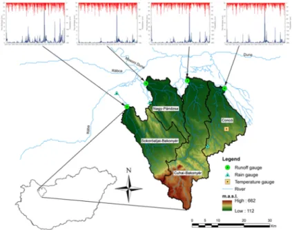
In the Little Hungarian Plain four basins were selected for evaluation; Concó, Cuhai-Bakonyér, Nagy-Pándzsa, and Sokoróaljai-Bakonyér (Fig. 1). Cuhai-Bakonyér is the largest catchment, and its major creek is Cuha. This region is one of the richest parts of Hungary in both surface and subsurface water resources. The Danube and its tributaries are the main water bodies here. This section of the Danube has mainly lower course characteristics; depositing sediment, forming islands and reefs. The Rába River is the largest tributary of the Danube, originating in Austria and flowing into the Mosoni-Danube in Győr, then into the Danube in Gönyü. Other major tributaries are;
Marcal, Rábca, and Répce. Two of the study basins, Sokoróaljai-Bakonyér and the Nagy-Pándzsa have streams connecting into the Rába River upstream from Győr.
Downstream from where the Rába meets the Danube, the other two basins join directly into the Danube river; first the Cuhai-Bakonyér, then Concó. Cuha originates in the Bakony mountains, which is also the highest part of the study area. Concó and its smaller tributaries are originating from the north-eastern foothills of the Bakony mountains. Nagy-Pándzsa and Sokoróaljai-Bakonyér originate from the north-western foothills of the Bakony mountains. The catchment outflow locations were determined based on the stream gauge locations.
The major part of the Little Hungarian Plain and the study area is covered with fluvial sediments of the Danube and Rába rivers [10]. In some locations, the thickness of the sediment reaches several hundred meters. In the south, the area is bordered by the Transdanubian Range, one of its subdivisions is the Bakony Mountains, where mostly
Pannonian (Upper Miocene) clastic sediments occur. At the foothills of the Bakony, smaller basalt bodies can be found. In the Cuha basin, all of the listed soil types can be found. In the southern part, where the Bakony Mountains are located, mainly dolomite and marl occurs, while in the central part, clay is more dominant. Toward the north, at the downstream end of the Cuha stream, river sediment and clay are the two main soil types. The Sokoró basin has a similar geological structure; the southern part of the basin is mainly dolomite, and in the middle and northern part, clay and river sediments become more dominant. The Concó and the Pándzsa basins have a different structure, since the upstream part of the basins start at the foothills of the Bakony. In the Concó basin, only clay, loess, and river sediment can be found. Two clay varieties can be found throughout the basin. In the Pándzsa basin, loess and clay are present; however, river sediment is the dominant geological formation.
Fig. 1. Location of the study area, including the runoff, precipitation, and temperature gauges and precipitation-runoff time series for 2000-2015.
Time series are included to show the rainfall-runoff relations.
In 2010 a flood occurred in every watershed. A smaller flood happened in 2013
The watersheds delineated with Geographical Information System (GIS) were obtained from the North-Transdanubian Water Directorate then further parameters were calculated by using GIS software. The terrain in all basins generally transitions from hilly-mountainous in the southern regions to undulating lowland and finally flat plains in the northern regions. The elevations range from 662 m.a.s.l. to 112 m.a.s.l. The largest catchment is Cuhai-Bakonyér with 484 km2, and the two smallest are Concó (281 km2), and Nagy-Pándzsa (262 km2).
Data
Data used in this study can be categorized into three main groups:
1) streamflow and precipitation data for the period 1 January 2000 - 31 December 2015 received from the North-Transdanubian Water Directorate;
2) climate, meteorological and transpiration data for the period 1 January 2000 - 31 December 2010 from the CARPATCLIM database and 1 January 2011 - 31 December 2015 provided by the National Weather Service;
3) basin data describing topography, land cover, soil properties, and geology from the Hungarian Academy of Science Institute for Soil Sciences and Agricultural Chemistry Agrotopo database, and the European Environment Agency Corine database. The final dataset is a 16-year long dataset for every catchment 1 January 2000 - 31 December 2015.
3. HEC-HMS model development
In the HEC-HMS model, hydrologic elements can be connected in a network simulating the structure of a watershed. Processes are organized into five main components; meteorological, rainfall loss, surface runoff, base-flow and routing. For continuous calibration and validation, the HMS-SMA model was used. The Soil Moisture Accounting (SMA) algorithm divides the potential path of rainfall on a basin into five zones, as shown in Fig. 2, [11].
Fig. 2. Soil moisture accounting model for the study area.
Shaded part is not included in model
The runoff process in the HMS-SMA model starts with precipitation. Precipitation can fall on the canopy vegetation or land surface. Some of the water returns to the atmosphere during evapotranspiration process. The Priestley-Taylor [12] model was
selected for evapotranspiration. During storm events evaporation is limited. A certain part of the precipitation falls through canopy, where it joins the water which fell directly on land surface. In the model the canopy evapotranspiration rate, ETc (mm) is calculated as
ET0 K
ETc= c⋅ , (1)
where Kc is canopy interception (-); ET0 is potential evapotranspiration (mm). Each vegetation cover has a different Kc value, and usually has a seasonal variation as well.
The Kc distribution within a year was assumed to be constant [13]. The inter-annual distribution of Kc values were obtained from a previous Hungarian study by Nagy [2], and are shown Fig. 3a.
Depending on the soil type, ground cover, and starting soil moisture conditions, the water may either pond or infiltrate. The infiltrated part of water is then stored temporarily in the upper layer of soils, and can rise by capillary action toward the surface and evaporate, or percolate vertically downward into the groundwater layer. The movement in the groundwater is slower, but will also reach the stream. Soil storage accounts for water that can be removed from the top soil layer by percolation or evapotranspiration. Soil Storage (SS) capacity in the model is determined by calculating the difference between the water content at saturation, θs and the water content at the wilting point, θr. Soil storage is partitioned into a tension zone component with no percolation and an upper zone component with percolation and evaporation. The Tension zone Storage (TS) is determined in the model by calculating the difference between the water content at field capacity (set to 0.33 bar suction) and wilting point (Fig. 3b). The values necessary to compute the moisture curves were obtained from previous Hungarian studies [14], [15]. The final calibrated parameters are presented in Table I.
a) b)
Fig. 3. a) Canopy interception rate and b) soil moisture curve
From the loss component, effective rainfall contributes to surface runoff and infiltration to groundwater flow in aquifers. For surface runoff, the Clark unit hydrograph method was used. For the base-flow component a linear reservoir base-flow
model was applied, which was used in conjunction with the SMA model. The channel routing component was not used.
Table I
Calibrated parameters
Parameter description Concó Cuha Pándzsa Sokoró
Soil parameters- SMA
Surface storage (mm) 30 45 40 30
Max. infiltration (mm/hr) 5.3 5 3 3
Soil storage, SS (cm3/cm3) 510 400 335 295
Tension-zone storage, TS (cm3/cm3) 160 60 260 140
Soil percolation rate (mm/hr) 0.01 0.008 0.006 0.01
Groundwater storage, GS (mm) 15 15 15 15
Groundwater percolation rate, TP (mm/hr) 0 0 0 0
Groundwater coefficient, TC (hr) 50 55 55 55
Linear base-flow
Linear reservoir coefficient, RTC (hr) 200 200 200 800
Linear reservoir (no) 1 1 1 1
Surface flow Clark Parameters
Time of concentration (hr) 12 24 30 15
Storage coefficient (hr) 50 120 150 82
4. Calibration and validation
A single basin model with four components was used for each basin in HEC-HMS.
The model was calibrated and verified for two non-overlapping 8-year periods of daily runoff data. A typical split-sample test proposed by Klemeš [16], was applied i.e. the model was calibrated for the period 2008-2015 and validated on 2000-2008, and finally evaluated for the 2000-2015 time period. The systematic manual calibration relied on the initial estimates of the input parameters. The output from the manual calibration was assessed by flow comparison graphs, and statistical goodness-of-fit measures, the Nash- Sutcliffe Efficiency (NSE) and the Kling-Gupta Efficiency (KGE).
Final model parameters were selected based on manual calibration by optimizing NSE and KGE and minimizing the error in volume (V%). The most important statistical measures were NSE and KGE. The Nash and Sutcliffe model efficiency value was determined as,
( )
( )
∑ −
∑ −
−
= 2
ˆ 2 1
Q Q
Q NSE Q
t t
t , (2)
where Qˆt is the predicted runoff at time t, Qt is the measured runoff at time t, and Q is the average observed runoff over a period of time. NSE can range between 1 and any negative number. One means perfect prediction, while zero means that the prediction is
no better than the average of the observed data. A negative value of NSE means poor prediction.
The Kling-Gupta Efficiency (KGE) index is estimated by,
(
1)
2(
1)
2(
1)
21− − + − + −
= cc Alpha Beta
KGE , (3)
where cc is the Pearson correlation coefficient between the measured (Qt) and predicted (Qt) runoff; Alpha is the relative variability in the predicted and measured values (equal to the ratio of standard deviation of predicted flow over the standard deviation of measured flow); and Beta is the ratio of the means of predicted and measured flows.
This method allows for a multi-objective assessment of the model performance, by decomposing the coefficient of determination in terms of mean bias, variability bias and correlation. Values close to one indicate a perfect fit, and decreasing values indicate decreasing model performance. Table II shows calibration results using the statistical performance measures selected for the model evaluation at the basins.
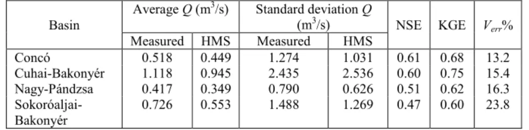
Table II
Statistical measures of calibration
Basin
Average Q (m3/s) Standard deviation Q
(m3/s) NSE KGE Verr% Measured HMS Measured HMS
Concó 0.518 0.449 1.274 1.031 0.61 0.68 13.2
Cuhai-Bakonyér 1.118 0.945 2.435 2.536 0.60 0.75 15.4 Nagy-Pándzsa 0.417 0.349 0.790 0.626 0.51 0.62 16.3 Sokoróaljai-
Bakonyér
0.726 0.553 1.488 1.269 0.47 0.60 23.8
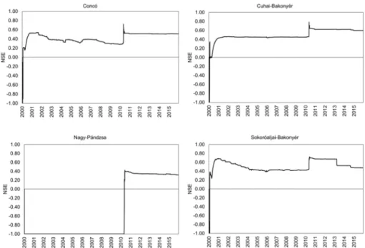
The means are under-predicted by the model and the standard deviations are less than the measured values. The statistical parameters, NSE, and KGE are higher for Concó, and Cuhai-Bakonyér, than for Nagy-Pándzsa, and Sokoróaljai-Bakonyér. Error in volume estimate is acceptable at less than 20%; only Sokoróaljai-Bakonyér has 23.8% error of volume. The calibration process was improved with the expanding- window error analysis. During calibration, the model performance was evaluated cumulatively throughout the entire time period as well. With this method NSE and KGE were calculated from the start of the simulation up to the current time step. This was repeated until the end of the simulation. Fig. 4 and Fig. 5 show the final distribution of NSE and KGE statistics for the calibration period. Looking at the NSE values over time, initial conditions dominated the first-year error and statistics results. During the second year, the statistics are improving. Due to high rainfall events in 2010 all basins show a large jump in the statistics, and after this year the statistics do not change significantly;
the NSE values are close to 0.60 in every basin. Sokoróaljai-Bakonyér behaves differently than the other basins; after 2010, the model works with NSE of 0.80, however in 2013 a change happens and the value drops to 0.60.
Fig. 4. Nash-Sutcliffe efficiency of calibration period.
Values below -1.0 assumed as -1.0 to show continuity
Fig. 5. KGE of calibration period
KGE values behaved differently than NSE, and gave us even more information on the division of errors since the three components of KGE were plotted. The cause of the lower KGE values in the first years is different for each basin.
At the Concó and Nagy-Pándzsa basin alpha is too high, which means that the standard deviation is over predicted. At the Cuhai-Bakonyér basin both alpha and beta are high, which means that both standard deviations and means are overestimated. After the first few years the parameters become stable in Concó, Cuhai-Bakonyér and Nagy- Pándzsa sites, with values close to 0.70. Sokoróaljai-Bakonyér has the same properties as when evaluating NSE; until 2010 KGE is stable, then some change occurred in the model and KGE became higher. There is another change also, at the end of 2014, when the value becomes lower. An interesting result is that in Nagy-Pándzsa and Sokoróaljai- Bakonyér site NSE and KGE are behaving oppositely after 2010; when NSE is increasing, KGE is decreasing. After the calibration, validations were performed for the period 2000-2015. Table III shows validation results using the statistical performance measures selected for the model evaluation at the basins.
Table III
Statistical measures of validation
Basin
Average Q (m3/s) Standard deviation Q
(m3/s) NSE KGE Verr% Measured HMS Measured HMS
Concó 0.400 0.400 0.968 0.776 0.51 0.66 0.1
Cuhai-Bakonyér 0.817 0.740 1.834 1.897 0.60 0.77 9.4 Nagy-Pándzsa 0.280 0.276 0.587 0.490 0.32 0.57 1.6 Sokoróaljai-
Bakonyér
0.549 0.513 1.154 0.944 0.48 0.64 6.5
Looking at the statistical measures, means are underestimated by the model except Concó, where match was perfect. The standard deviations are less than the measured except Cuhai-Bakonyér. The NSE and KGE are highest for Cuhai-Bakonyér and close to each other for Concó and Sokoróaljai-Bakonyér. For Nagy-Pándzsa, the values are lowest. Volume error is acceptable; less than 10%. During validation, we evaluated the performance during the whole-time period as well. Fig. 6 and Fig. 7 are showing the final distribution of NSE and KGE for the validation period.
Based on the results, NSE is acceptable in Concó, Cuhai-Bakonyér and Sokoróaljai- Bakonyér basins. After one year, Cuhai-Bakonyér became stable, while in Concó and Sokoróaljai-Bakonyér there are slight uncertainties until 2010. Nagy-Pándzsa is more variable. Until 2010, the NSE is less than -1.0, however from 2010 the model starts to work better with NSE 0.30 to 0.40.
KGE values indicate closer agreement. In Concó and Cuhai-Bakonyér basins, the values are stable and after 2010 the model becomes slightly better. In Nagy-Pándzsa, KGE ranges between -1.0 to 1.0 over the 16-year period, and there are two main changes; the first in 2006 and the second in 2010. Sokoróaljai-Bakonyér behaves differently; KGE decreases until 2005, then it starts to increase in three steps.
Fig. 6. Nash-Sutcliffe efficiency of validation period.
Values below -1.0 assumed as -1.0 to show continuity
Fig. 7. KGE of validation period
5. Discussion of results
Possible explanation for these behaviors was investigated and it was found that in the Nagy-Pándzsa basin a stream-flow revitalization program ran from 2009 to 2011.
During this time the river received a concrete channel lining and storage elements and water control infrastructures were built. In Sokoróaljai-Bakonyér, starting with 2010 there was insufficient source for river maintenance, especially for cutting. Based on Water Directorate data, the planned cuttings were almost never made at time. One of the most important conclusions is that one should be critical with the model efficiency parameter (NSE) coming from the analysis, because it is only the final value of the modeling process. It is more important to evaluate the changes in the parameter over time.
6. Conclusion
The HEC-HMS model was used for daily flow prediction. The model was calibrated between the 2008-2015 time period and validated between 2000 and 2015. The results were evaluated using graphical and statistical measures. Three statistical measures were selected for evaluation; NSE, KGE and the continuously expanding window method.
With the continuously expanding window, statistical measures were evaluated not only at the final time step, but during the whole assessment period as well.
The NSE statistics resulted with values between 0.3 and 0.6, and KGE from 0.5 to 0.8. Concó and Cuhai-Bakonyér had highest statistics, while Nagy-Pándzsa lowest.
Finally, the expanding window method was used to evaluate the modeling effort.
By observing the continuous statistical measurements, one can detect changes in either meteorological, watershed characteristics or errors in data collection. The 2010 flood had a significant impact on the watershed behavior at all basin, causing a sudden jump in the error analyses and improving statistical performance at all watersheds. The size of the jump is related to the changes in watershed storage characteristics, but further investigations are required to determine the cause of this behavior. The Sokoróaljai-Bakonyér resulted in another interesting distribution of errors; during the whole-time period the KGE statistics were never stable, especially before 2010.
The other conclusion is that one has to be careful with the applied statistical measure. In the Nash and Sutcliffe model efficiency (NSE) models mean square error is normalized with the standard deviation of observed flows, while Kling-Gupta efficiency (KGE) allows for a multi-objective assessment of the model performance, by decomposing NSE in terms of mean bias, variability bias and correlation as separate criteria to be optimized.
It was observed, that better model and better statistics can be achieved when during calibration and validation process one assess the continuous distribution of statistical measures over time, instead of only the final statistics.
Acknowledgement
The Authors are thankful to North-Transdanubian Water Directorate for data. This work was undertaken as part of a project founded by the EFOP-3.6.1-16-2016-00017.
References
[1] Koch R., Bene K. Continuous hydrologic modeling with HMS in the Aggtelek karst region, Hydrology Research, Vol. 1, No. 1, 2013, pp. 1–7.
[2] Nagy E. D., Torma P., Bene K. Comparing methods for computing the time of concentration in a medium-sized Hungarian catchment, Slovak Journal of Civil Engineering, Vol. 24, No. 4, 2016, pp. 8–14.
[3] Legates D. R., McCabe G. J. Jr. Evaluating the use of ‘goodness-of-fit’ measures in hydrologic and hydro-climatic model validation, Water Resources Research, Vol. 35, No. 1, 1999, pp. 233–241.
[4] Nash J. E., Sutcliffe J. V. River flow forecasting through conceptual models, Part I, A discussion of principles, Journal of Hydrology, Vol. 10, No. 3, 1970, pp. 282–290.
[5] Krause P., Boyle D. P., Bäse F. Comparison of different efficiency criteria for hydrological model assessment, Advances in Geosciences, Vol. 5, 2005, pp. 89–97.
[6] Asadzadeh M., Leon L., Yang W., Bosch D. One-day offset in daily hydrologic modeling:
An exploration of the issue in automatic model calibration, Journal of Hydrology, Vol. 534, 2016, pp. 164–177.
[7] Guse B., Pfannerstill M., Gafurov A., Kiesel J., Lehr C., Fohrer N. Identifying the connective strength between model parameters and performance criteria, Hydrology and Earth System Sciences, Vol. 21, 2017, pp. 5663–5679.
[8] Lachance-Cloutier S., Turcotte R., Cyr J. F. Combining stream-flow observations and hydrologic simulations for the retrospective estimation of daily stream-flow for un-gauged rivers in southern Quebec (Canada), Journal of Hydrology, Vol. 550, 2017, pp. 294–306.
[9] Gupta H. V., Kling H., Yilmaz K. K., Martinez G. F. Decomposition of the mean squared error and NSE performance criteria: Implications for improving hydrological modeling, Journal of Hydrology, Vol. 377, No. 1–2, 2009, pp. 80–91.
[10] Budai T., Csillag G., Kercsmár Z., Selmeczi I., Sztanó O. Surface geology of Hungary (Explanatory notes to the Geological map of Hungary, Geological and Geophysical Institute of Hungary, Budapest, 2015.
[11] Hydrologic modeling system HEC-HMS: Technical reference manual, Davis, California, U.S. Army Corps of Engineers, Hydrologic Engineering Center, 2000.
[12] Priestley C. H. B., Taylor R. J. On the assessment of surface heat flux and evaporation using large-scale parameters, Monthly Weather Review, Vol. 100, No. 2, 1972, pp. 81–92.
[13] Allen R., Pereira L., Smith M., Raes D., Wright J. Coefficient method for estimating evaporation from soil and application extensions, Journal of Irrigation and Drainage Engineering, Vol. 131, No. 1, 2005, pp. 2–13.
[14] Kozma Z., Ács T., Koncsos, L. Hydrological modeling of the unsaturated zone - evaluation of uncertainties related to the FAO soil classification system, Pollack Periodica, Vol. 8, No. 3, 2013, pp. 163–174.
[15] Murinkó G., Bene K. Hydrologic modeling of the loess bluff in Dunaújváros, Hungary, Pollack Periodica, Vol. 12, No. 1, 2017, pp. 3–15.
[16] Klemeš V. Operational testing of hydrological simulation models, Hydrological Sciences Journal, Vol. 31, No. 1, 1986, pp. 13–24.