Data reduction and univariate splitting — Do they together provide better corporate bankruptcy prediction?

(1)

Data reduction and univariate splitting – do they together provide better corporate bankruptcy prediction?

Abstract

Discussion on methodological problems of corporate survival and solvency prediction is living its renaissance in the era of financial and economic crisis. Within the framework of this article the most frequently applied bankruptcy prediction methods are competed on a Hungarian corporate database. Model reliability is evaluated by ROC curve analysis. The article attempts to answer the question whether the simultaneous application of data reduction and univariate splitting (or just one of them) improves model performance, and for which methods it is worth applying such transformations.

JEL classification codes C33; C45; C51; C52; G33

Keywords

bankruptcy prediction, classification, univariate splitting, ROC curve analysis, logistic regression, decision tree, neural networks

1. Introduction

For many years the number of companies becoming insolvent has been increasing in the majority of Central and Eastern European countries, and the crisis has substantially boosted this tendency. Accordingly an escalating interest can be noticed towards multivariate

(2)

statistical bankruptcy prediction models in business life. Discussion on methodological problems of corporate survival and solvency prediction is living its renaissance.

Corporate survival and solvency prediction is a complex problem. Researching this field is encumbered and at the same time challenged by the ascertainments that no unified theory exists to explain and understand organizational survival, no method exists to guarantee unambiguous survival prediction, and it is noticeable that different empirical researches result in contradicting conclusions. Throughout the 40-year-history of multivariate statistical bankruptcy prediction no agreement was made among scholars in the field what explanatory variables provide the most reliable prediction. Consequently competitive and supplementary theoretical and methodological approaches coexist in the field.

For financial ratio based multivariate statistical corporate bankruptcy prediction discriminant analysis has been widely applied since the pioneer work of Altman (1968), which has been more and more replaced since the 1980s by logistic regression analysis (Ohlson, 1980). Decision trees (Frydman, Altman, Kao, 1985) also began to spread in the 1980s. Since the 1990s the neural networks have given a boost to improve the reliability of solvency forecast models. Neural networks were firstly applied for corporate bankruptcy forecasting by Odom, Sharda (1990).

Several empirical researches were accomplished to compare the performance of different bankruptcy forecast methods, a summary analysis is provided inter alia in Virág, Kristóf (2005) and Xu, Chen, Haitao (2011). According to the majority of the authors neural networks overperform the traditional methods; whereas some authors (i.e. Laitinen, Kankaanpaa, 1999) arrived at the provocative conclusion that all methods provide similar performance.

The aim of this article is to compete the most frequently applied bankruptcy forecast methods on a Hungarian corporate database. Besides predicting the solvency status, probability of survival values are forecasted for each company by each method. Within the

(3)

framework of empirical research the performance of logistic regression, decision trees and neural networks is compared.

Beyond developing models using the original continuous financial ratios two transformations were applied with the hope to improve predictive power. The first one was principal component analysis to preserve explained variance of linear correlated variables and at the same time handle multicollinearity. The second one was chi-square based univariate decision trees to derive categorical variables from continuous ones with the aim to find relatively homogeneous risk categories. It was also tried to accomplish the two transformations together by splitting the factors.

Our hypothesis was that data reduction and univariate splitting together provide better prediction than the pure application of the methods without such transformations, and in each case neural networks perform better than logistic regression or decision trees.

2. The frameworks of empirical research

The traditional objective of corporate survival and solvency forecasting is to find out with the highest reliability whether a company is expected to go into bankruptcy within one year after the turning day of its last annual report, and to estimate probability of survival values for each company.

2.1. Size and breakdown of the sample, explanatory variables

To ensure the applicability of models on any company it was set as a requirement towards data collection that data available for modeling has to come from public annual reports and company register. Balance sheets and profit&loss statements from 2004 were collected. The

(4)

sample contains 504 companies from which 437 are solvent and 67 are insolvent. This magnitude of observations is statistically manageable; furthermore many companies and small/middle banks usually possess clientele of that size, accordingly it can be argued to be a typical modeling problem in business life.

The empirical research equates corporate failure to the legal possibilities of insolvency, namely the declaration of bankruptcy procedure, liquidation or winding up. The legal category of insolvency was not differentiated later. Solvent observations were denoted by 0 and insolvent ones by 1.

Explanatory variables were defined using information expressing corporate size, industrial classification, profitability, turnover, liquidity, capital structure, debt, cash flow and annual growth. Variable selection was preceded by an in-depth professional analysis. Altogether 31 financial ratios were defined. Calculation formulae of the financial ratios are summarized in Appendix 1.

Data collection was followed by data preparation for modeling. It is often more difficult than modeling itself, since unpredicted problems with observations and/or variables might emerge. The calculation of two financial ratios was limited by the zero value of the denominator. From the companies in the sample 6 had zero inventory and 11 zero trade receivables, thereby making it impossible to calculate inventory turnover and trade receivables turnover ratios. This problem was solved – by considering data mining experiences in the field of financial modeling (Han, Kamber, 2006) – in a way that missing inventory turnover values were substituted by the median value of other observations, and the missing trade receivables by the 97.5% percentile value as a truncated maximum.

It was substantially more difficult to use three financial ratios distorted by double negative division. The coexistence of negative nominator and negative denominator concerned return on equity (ROE) in 28 cases, operating profit growth in 74 cases, and profit after tax growth

(5)

in 67 cases. In the case of ROE it means that in the sample there are 28 companies, the liabilities of which first exceed their total assets and second they closed the financial year with loss, and despite these facts the ratio shows a positive profitability. This problem was naturally characteristic to the insolvent observations. As for the growth ratios of the two profit categories companies having negative profit both in the previous and in the actual year (even with further worsening operating or after tax profit in the actual year) could be wrongly characterized by positive growth. In such case a widely used data mining technique is to replace the ratio-value of companies having double negative items with the minimum ratio- value of the other companies, however, considering the small sample and the relatively large number of affected companies these three ratios were discarded from the empirical research.

Distribution of companies in the sample could be classified into 10 national economic branches, 41 industries and 164 special-branches, the latter means four digit Standard Sectoral Classification of Economic Activities (SSCEA) code breakdown. Manufacturing companies represented themselves in the greatest share within the sample.

Still before the 1990s some scholars (like Platt, Platt, 1990) extensively dealt with the problem how corporate ratios and industry performance together influence the likelihood of insolvency. Since then the most efficient bankruptcy prediction models have been applying industrial distinction. To compare financial ratios of companies operating in different industries the differences from special-branch averages were considered instead of pure financial ratio-values. The correction was carried out by the following formula:

Individual ratio value – Special-branch average value Special-branch average value (1)

Correction by special-branch averages ensures the comparability between companies having pretty different fields of activities. From this point empirical research does not refer to

(6)

the individual financial ratio-values, but to their variance from their special-branch averages.

Thereby time stability of the models is improving, since better or worse performance compared to the averages might remain a relevant perspective to evaluate insolvency after several years.

To validate models and avoid overtraining the sample was partitioned on the basis of simple random selection to a 75% training and a 25% testing set. It is a thumb rule of bankruptcy prediction that if the modeling database (training set) contains less than 50 insolvent observations, it is not reasonable to apply multivariate statistical methods (Engelman, Hayden, Tasche, 2003). This requirement was barely met in the empirical research, as within the training sample containing 371 observations 320 were solvent and 51 were insolvent, and within the testing sample containing 133 observations 117 were solvent and 16 were insolvent.

2.2. Data reduction, univariate splitting

Data reduction was carried out by principal component analysis (PCA), which is commonly used in financial modeling (see i.e. Hu, Ansell, 2007). PCA constructs uncorrelated components (factors) from the linear correlating variables. The essence of the procedure is that some components can explain a great share of the total variance of the variables; thereby it is enough to have fewer dimensions for modeling. PCA is proven to be able to handle multicollinearity and reduce data (Krzanowski, 2000). For applying the procedure it is key to decide on the number of components, which is most frequently defined with the help of eigenvalues above a certain threshold (Kovács, 2006). Eigenvalues show the aggregation capability of input data variances for each component. Factors were constructed by considering the following criteria:

(7)

 strong and significant linear correlation exists between variables;

 from financial viewpoint variables have similar meanings;

 eigenvalue is higher than 1;

 Kaiser-Meier-Olkin (KMO) measure of sampling adequacy is at least 50%;

 the factor is significant using the Bartlett-test.

Altogether seven factors were derived. Appendix 2 summarizes the factor equations together with eigenvalues, total explained variances and KMO values. All the factors were significant according to the Bartlett-test.

Univariate splitting was accomplished by the Chi-squared Automatic Interaction Detection (CHAID) method. CHAID is a classification method for building decision trees by using chi- square statistics to identify optimal splits (Kass, 1980). The procedure first examines the cross tabulations between each of the independent variables and the outcome, and tests for significance using a chi-square independence test. If more than one of these relationships is significant, the method will select the predictor which is the most significant. If a predictor has more than two categories, these are compared, and categories that show no differences in the outcome are collapsed together. This is done by successively joining the pair of categories showing the least significant difference. This category-merging process stops when all remaining categories differ at the specified testing level.

CHAID is excellent to explore the relationship-characteristics between the target variable and the explanatory variables one by one, and is able to select the variable which in itself has the strongest predictive power (Frydman, Altman, Kao, 1985). The essence of this procedure is to form groups, which most differ from each other considering solvency. It was reasonable to build decision trees for nineteen original variables and six PCA factors. The trees can be

(8)

interpreted by examining the distribution of solvent and insolvent observations within nodes.

The top node incorporates the total sample having 13.3% insolvent rate. A category is regarded as risky if the insolvent rate substantially exceeds 13.3%, and not risky in case of substantially lower insolvent rate. Financial ratio thresholds are illustrated above the nodes.

To make modeling easier the belonging to the categories was denoted by dummy variables, hence the CHAID split models exclusively contain 1/0 values. It was expected that the application of univariate decision trees results in a better predictive power.

2.3. Applied forecast methods

The following points briefly analyze the application assumptions, advantages and drawbacks of the applied multivariate statistical forecast methods. It was planned to apply discriminant analysis as well, however, according to our experience, this method results in a poor performance when considering categorical variables.

2.3.1. Logistic regression analysis (Logit)

Logistic regression analysis is a widely used approach to model relationships between explanatory variables and the likelihood of a binary response (Chatfield, Collins, 2000). The procedure orders probability of survival/bankruptcy values to the weighted independent variables by fitting a logistic regression function estimated by the maximum likelihood method.

The advantages of the method are robustness, exact appearance of relative contributions and easy interpretation. Drawbacks are the possibility of small-sample biasedness, the sensitivity to outliers, the accidental emergence of multicollinearity and the application of

(9)

predefined function-type. If the solvency rate of the sample differs from that of population, the estimated probability of survival values might be modified by probability-calibration in such a way that the average probability of survival value equals to the desired rate, at the same time the order of probabilities estimated for the observations must be preserved.

2.3.2. Decision trees

The procedure attempts to build a decision tree by iteration, using univariate partitioning, setting simple decision rules, and constructing branches (Kass, 1980). The aim is to establish the most homogeneous classes. The algorithm establishes branches as long as it finds partitioning variables. The first partitioning variable is found at the top of the tree. The roots of tree mean the solvent and insolvent classification after the partitioning.

The advantages of the method are the few application assumptions and the obvious interpretation of the decision rules. Drawbacks are the accidental appearance of overtraining, the assumption of discrete classification capability and non-overlapping between the groups.

No statistical testing can be carried out on the model, and the relative contribution of variables cannot be unambiguously determined. Probability of survival values can be estimated on the basis of decision rules.

2.3.3. Neural networks (NN)

Neural networks are information processing systems constructed on the basis of biological neural systems having the capability to operate simultaneously in a shared way (Gurney, 1996). Networks consist of interconnected, parallel functioning neurons, and gain their problem-solving capability by learning. Fundamental components of neural networks are the

(10)

elementary neurons, which are organized in layers. Weighting of the networks is established through the learning process.

The advantages of the method are the few application assumptions, the intelligent learning of relationships and the universal approximation feature. Drawbacks are the black box problem, the accidental appearance of overtraining, arriving at local minima, the indirect determination of relative contributions and the inability to carry out statistical tests (Perez, 2006). Neural networks can automatically estimate probability of survival/bankruptcy values.

If the solvent rate of the population and the sample substantially differs from each other, probability-calibration might be necessary.

It has been proven in some earlier publications (see i.e. Ghiassi, Saidane, Zimbra, 2005) that dynamic neural network models provide more accurate forecast and perform significantly better than traditional neural networks, like feedforward or backpropagation. For that reason the neural network model in the empirical research was trained by the exhaustive prune technique (Huang, Saratchandran, Sundararajan, 2005). With exhaustive prune, network training parameters are chosen to ensure a very thorough search of the space of possible models to find the best one.

2.4. Analytical aspects, reliability-examination methods

Theoretical and practical requirements demand the direct comparability of bankruptcy prediction models constructed by different methods. This expectation can only be met if input data of modeling is exactly the same for each method, model outputs are measured on the same scale in the same intervals, and model performance is evaluated by the same reliability- examination methods. Identical input information is guaranteed in the empirical research.

(11)

It was drawn as a fundamental criterion towards forecast methods that all the three must result in probability of survival values between 0 and 1. Logistic regression and neural networks automatically meet this requirement. In case of decision trees probability of survival values were estimated from the classification capabilities of decision rules.

The requirement to determine the significance/relevance of certain variables presumes the exact measurement of relative contribution of the variables. It is easy to see that this measurement problem occurs when evaluating neural networks. The empirical research measured the importance of input neurons with the help of sensitivity analysis. In case of decision trees it can only be concluded that the first partitioning variable has the highest contribution to the model performance.

It can be drawn as a general validity that reliability-examination is an equal-ranking task to making forecast (Gáspár, Nováky, 2002). In case of bankruptcy prediction it should not be hauled up from predictions whether they took place in reality, but whether they provided appropriate information to make the necessary decisions (e.g. credit appraisal). It is expected from reliable bankruptcy models that they promote to avoid potentially unfavorable situations.

Model validation reveals how well the models are performing (Medema, Koning, Lensink, 2009).

Reliability of forecast models is evaluated using the Receiver Operating Characteristic (ROC) curve analysis. ROC curve is a useful analytical tool to evaluate the performance of classification rules in case of binary output and estimated probability values or scores (Stein, 2005). The ROC curve examines how reliable the estimated probabilities reflect the belonging to the output categories, if the a priori classification is known. The curve considers the observations in the sample in the sequence of their estimated probability of survival/bankruptcy. Horizontal axis represents the cumulative distribution of solvent and vertical axis the cumulative distribution of insolvent observations. The reference of ROC

(12)

curve is the 45°-line, which represents random guessing. The evaluation of a bankruptcy model is better if its curve better drifts apart from the 45°-line (Agarwal, Taffler, 2007).

The area under ROC curve (AUROC) is an objective statistical indicator. If the AUROC exceeds 50% then it has an added value compared to random guessing. Model having higher AUROC means better model. It is an established custom of ROC analysis to estimate the 95%

confidence interval of AUROC. When evaluating bankruptcy models the ROC curves and AUROCs of the total sample and the testing set are considered for each forecast method. It is also usual to evaluate model performance using the GINI coefficient.

3. Developed models

Bankruptcy prediction models were elaborated using the observations and variables after industrial mean correction. Each method was applied using the following strategies:

 entering the original variables;

 entering the original variables together with continuous PCA factors;

 entering the CHAID split original variables;

 entering the CHAID split original and PCA variables.

3.1. Logistic regression based models

In this empirical research the logistic regression models were constructed using the forward stepwise procedure. Variable selection was carried out by using the Wald entry and removal criteria. The entry criterion was defined as 5% and the removal criterion as 10%

probability value. Model testing was carried out with the help of the asymptotic ² test based

(13)

Omnibus-test. Both the continuous financial ratio and the PCA model contained indebtedness, size and cash flow indicators besides the constant. The CHAID split models also entered profitability and growth ratios instead of cash flow ratios.

Table 1. Main features of the logistic regression models

Explanatory variable  Standard

error Wald- test p-

value Model using the original variables

Long term indebtedness -.830 .257 10.429 .001

Indebtedness 2.084 .358 33.816 .000

Net_revenue -8.118 1.721 22.257 .000

Cash_flow_liabilities -.073 .031 5.479 .019

Constant -5.132 .656 61.119 .000

Model significance: ²=126.6 (degree of freedom: 4), p=0.000 Model using the PCA factors

Long term indebtedness -.733 .247 8.804 .003

Indebtedness 1.836 .353 27.108 .000

PCA_SIZE -1.131 .235 23.118 .000

PCA_CASH_FLOW -.651 .249 6.817 .009

Constant -3.045 .309 97.014 .000

Model significance: ²=125.6 (degree of freedom: 4), p=0.000 Model using the CHAID split original variables

CHAID_ROA_1 -1.822 .525 12.068 .001

CHAID_FIXED_ASSETS_DEBT_1 -1.009 .515 3.841 .050 CHAID_REVENUE_GROWTH_2 1.414 .479 8.712 .003 CHAID_EBITDA_MARGIN_1 -2.541 .573 19.673 .000 CHAID_INDEBTEDNESS_1 2.065 .525 15.483 .000 CHAID_NET_REVENUE_1 -1.473 .551 7.154 .007 CHAID_CASH_LIQUIDITY_1 -1.831 .538 11.562 .001

Constant .904 .657 1.894 .169

Model significance: ²=171.2 (degree of freedom: 7), p=0.000 Model using the CHAID split original and PCA variables

CHAID_ROA_1 -1.909 .520 13.461 .000

CHAID_REVENUE_GROWTH_2 1.333 .469 8.097 .004 CHAID_PCA_LEVERAGE_1 -1.803 .520 12.014 .001 CHAID_EBITDA_MARGIN_1 -2.847 .573 24.671 .000 CHAID_INDEBTEDNESS_1 2.118 .508 17.401 .000 CHAID_NET_REVENUE_1 -1.747 .549 10.117 .001

Constant .631 .607 1.083 .298

Model significance: ²=169.7 (degree of freedom: 6), p=0.000

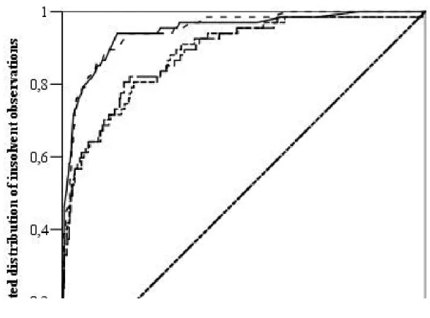
On the basis of the ROC curves it can be concluded that all the four models have favorable performance characteristics. The 88.5%-94.8% AUROC indicators show excellent

(14)

classification capabilities. All the ROC curves have sharp increasing sections in the beginning, proving that they can classify the most insolvent companies with very good accuracy.

Figure 1. ROC curves of the logistic regression models

It is also obvious that no clear distinction can be made between two-two models, namely between the two continuous and the two categorical models. The ROC curves often intersect each other and have very similar shapes. However, one thing is visible: both categorical models have better performance than the two continuous models. Hence it can be concluded on the basis of this empirical research that it is reasonable to apply univariate splitting in case of logistic regression, and factor analysis is not worth the trouble.

Table 2. Model performance indicators (n=504)

(15)

Model AUROC (95% confidence interval) GINI coefficient¹ LOGIT_ORIGINAL 88.5% (83.9% – 93.0%) 77.0%

LOGIT_PCA 88.5% (83.9% – 93.0%) 77.0%

LOGIT_CHAID 94.8% (92.2% – 97.5%) 89.6%

LOGIT_CHAID_PCA 94.6% (91.5% – 97.7%) 89.2%

Another thing which proves the better applicability of CHAID-split models is the performance-difference of the training and the testing sets, however, such results must be handled with caution, since the testing set involves only 16 insolvent observations. The two continuous models have 91.1% and 91.5% AUROC on the training set and only 80.7% and 79.7% on the testing set, whereas the two categorical models 95.6% and 95.4% on the training set and 92.3% and 91.5% on the testing set. Therefore the continuous models are rather overtrained, and cannot be applied effectively on new observations. This is another reason for using the CHAID split models in practice.

3.2. Decision tree based models

The decision tree models went through a pruning procedure to avoid overtraining. The pruning procedure attempts to accomplish risk-minimization by defining different closing nodes. Increasing the number of closing nodes usually reduces the risk of specialization to the training set, and improves the cross-validation features of the model.

Decision tree pruning could be influenced by different stopping rules, which prevent from the further splitting of certain branches. In the current empirical research the possibility of forming parent branch was set to the minimum 7% of the records within training set, and that of child branch was defined as minimum 5%. The models were constantly backtested on the testing set, and according to the results of tracking it was concluded that no more rigorous conditions were needed.

1 GINI = (2×AUROC) – 1

(16)

At the end of each decision rule classification can be done using the insolvent rates in the last nodes. The results can be interpreted as probability of bankruptcy/survival values.

According to the idiosyncrasies of decision trees as many different probability of survival values are ordered to the observations as many kind of decision rule combinations exist in the tree structure.

Appendix 3 summarizes the four decision tree models. In the first two models cash flow, size, liquidity, indebtedness, capital coverage and growth ratios were regarded as relevant² model variables, which is good from corporate financial viewpoints.

Modeling with the CHAID split variables the procedure is like binary splitting. Only one category of a given variable is considered in one simulation step, and interestingly always the first categories were found to be relevant splitting variables. In the CHAID split models EBITDA, cash flow, indebtedness, size, profitability, working capital and liquidity ratios were regarded as relevant model variables, which is very good from corporate financial perspectives.

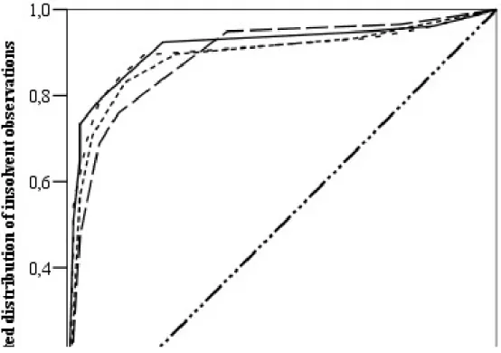
On the basis of the ROC curves it can be concluded that the continuous models have similar or somewhat better performance characteristics than the logistic regression models.

Performance indicators show very good classification capabilities. However, it is very hard to decide on the best decision tree model, since all the ROC curves intersect one another.

Figure 2. ROC curves of the decision tree models

2 term ’significance’ does not make sense in case of simulation procedures

(17)

Under such circumstances three viewpoints can be considered: first, which is the steepest curve in the section of the first twenty probability of survival percentiles demonstrating that this model classifies the most insolvent companies with the best accuracy, second, which has the greatest AUROC, and third, which model is least overtrained.

Table 3. Model performance indicators (n=504)

Model AUROC (95% confidence interval) GINI coefficient RPA_ORIGINAL 88.8% (85.1% – 92.6%) 77.6%

RPA_PCA 88.9% (84.8% – 92.9%) 77.8%

RPA_CHAID 89.8% (86.4% – 93.1%) 79.6%

RPA_CHAID_PCA 91.1% (87.9% – 94.3%) 82.2%

From all the three perspectives the decision tree containing categorical original and PCA variables is the best. The CHAID_PCA model has 94.2% AUROC on the training set and 86.4% on the testing set. The most overtrained model is the continuous PCA model (92.0%

AUROC on the training set and 78.4% on the testing set). Therefore it can be concluded on the basis of this empirical research that it is reasonable to apply both data reduction and

(18)

univariate splitting in case of decision trees, however, even the best model has slightly worse performance characteristics compared to the best Logit model.

3.3. Neural network based models

The neural networks were trained by the exhaustive prune technique. The exhaustive prune technique starts from a network containing all independent variables as input neurons and having a great number of neurons in the hidden layers. Weights initially take random values. In the training epochs the procedure attempts to exclude neurons having low explanatory power from the input and the hidden layers. During training final weights are estimated very thoroughly by trying and validating several network-structures simultaneously.

Temporarily it might be necessary to take back some neurons into the layers. This procedure has much more computation-requirements than the traditional procedures using predefined structure; however, according to experiences it provides the best results. To avoid overtraining weights estimated on the basis of training set are constantly backtested on the testing set. Final model weights are saved when achieving the highest classification accuracy on the testing set.

The relative contribution of neural network model variables can be estimated by sensitivity analysis. As a result of sensitivity analysis a value of importance between 0 and 1 is provided, where higher value means higher level of contribution to the predictive power of the model. Model variables are acceptable from corporate financial viewpoints in all the four neural network models.

Table 4. Neural network models and values of importance

Model variable Value of importance Model with original variables

(19)

Network structure: 5-2-1-1

Dynamic profitability ratio 0.6894

Indebtedness 0.5998

Working capital ratio 0.5678

Net revenue 0.5149

Capital coverage 0.2890

Model with PCA factors Network structure: 9-3-3-1

PCA_CASH_FLOW 0.7813

Indebtedness 0.7467

PCA_SIZE 0.4812

Current assets ratio 0.3743

ROA 0.2033

EBITDA profitability 0.1835

Capital coverage 0.1762

Leverage 0.1671

Dynamic liquidity 0.0954

Model with CHAID split original variables Network structure: 7-1-3-1

CHAID_ROA_1 0.1129

CHAID_INDEBTEDNESS_2 0.1067

CHAID_REVENUE_GROWTH_2 0.1065

CHAID_EBITDA_MARGIN_2 0.0925

CHAID_CASH_LIQUIDITY_2 0.0653

CHAID_LONG_TERM_INDEBTEDNESS_1 0.0596

Model with CHAID split original and PCA variables Network structure: 16-2-2-1

CHAID_ROA_1 0.0581

CHAID_LONG_TERM_INDEBTEDNESS_1 0.0571

CHAID_PCA_LEVERAGE_2 0.0426

CHAID_PCA_SIZE_2 0.0423

CHAID_DYNAMIC_PROFITABILITY_3 0.0406

CHAID_PCA_CAPITAL_3 0.0271

CHAID_PCA_LEVERAGE_1 0.0137

CHAID_PCA_SIZE_1 0.0097

CHAID_DYNAMIC_LIQUIDITY_1 0.0055

CHAID_PCA_CAPITAL_1 0.0036

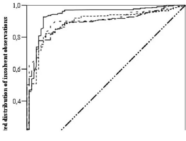
On the basis of the ROC curve analysis it can be concluded that the performance of three models practically cannot be distinguished, since the ROC curves intersect one another and the AUROC indicators have little difference: the two continuous models and the CHAID split

(20)

model. However, each model possesses good classification capabilities. The ROC curve of the CHAID_PCA model “covers” the others almost in the total probability of survival percentile range and has the highest AUROC, therefore this is the best model.

Figure 3. ROC curves of the neural network models

As far as overtraining is concerned the continuous PCA model shows the greatest sign to be overtrained, since its AUROC is 90.8% on the training set and 83.1% on the testing set.

The CHAID_PCA model provides the best result on the testing set (AUROC=87.7%).

Table 5. Model performance indicators

Model AUROC (95% confidence interval) GINI coefficient

NN_ORIGINAL 88.7% (84.8% – 92.6%) 77.4%

NN_PCA 89.1% (85.9% – 92.3%) 78.2%

NN_CHAID 89.6% (86.2% – 93.0%) 79.2%

NN_CHAID_PCA 93.5% (90.1% – 96.9%) 87.0%

(21)

On the basis of empirical research it seems that in case of neural networks it is advisable to apply together data reduction and univariate splitting. Furthermore it has to be also remembered that even the best neural network model underperforms the best logistic regression model.

4. Conclusions

Using the experiences of constructing twelve bankruptcy models on the same Hungarian corporate database it can be concluded that data reduction and univariate partitioning do make sense in the field of bankruptcy prediction. All the elaborated models are acceptable from corporate financial aspects, and all of them possess high classification power. On the basis of model performances it can be argued that univariate splitting adds more value to model improvement than data reduction.

On the basis of AUROC indicators a sequence can be set to the classification power of elaborated models. In this sense the two categorical logistic regression models are the best ones, and they are followed by the CHAID_PCA neural network model, and then comes the CHAID_PCA decision tree.

It is interesting to note that no difference can be reported between the reliability of the three forecast methods when using the original continuous variables despite the relatively small sample and the perceived superiority of neural networks in several other comparative empirical researches. It is also clear that based on this empirical research that PCA in itself does not substantially improve predictive power, and might result in more overtrained models.

Studying the stability of the developed models it can be asserted that the application of CHAID split categorical variables results in less overtrained models, hence more stable models can be developed with the help of univariate splitting.

(22)

The dilemma whether the simultaneous application of data reduction and univariate splitting can be recommended for modeling practitioners is not resolved unambiguously. It is reasonable to do so in the case of decision trees and neural networks, however, in case of logistic regression the CHAID splitting in itself has very favorable impact, and PCA does not have added value at all. The simultaneous application is mostly recommended for neural network practitioners.

In recent times the demand for bankruptcy prediction models has strengthened for several reasons. Corporate bankruptcy concerns the majority of stakeholders. Since bankruptcy is usually accompanied with high costs, it is the interest of the stakeholders to recognize the danger of bankruptcy in time. Negative tendencies in economic environment and the rapid improvement of corporate performance measurement have enhanced the research of bankruptcy reasons and the spreading of bankruptcy forecasting culture. Availability of financial information and recent achievements of quantitative sciences have given a boost to empirical researches in the field of bankruptcy forecasting. With the help of bankruptcy prediction models a reliable picture can be gained on the economic situation of the companies, and it is possible to estimate individual probability of survival values for the companies.

Application of bankruptcy models might reduce information asymmetry between investors and managers, and they can be extensively used for risk analysis. By constantly tracking significant and/or relevant financial ratios companies, creditors and other stakeholders might be able to recognize the danger of insolvency at an early stage.

Results achieved in this article provide practitioners with methodological guidelines, normative proposals and concrete modeling techniques. Being aware of the corporate insolvency tendencies in Hungary it is foreseeable that reliable bankruptcy forecasting will surely be needed in the short, mid and long run as well. Hence the knowledge about factors having impact on corporate survival and solvency, tracking of them and the capability to

(23)

distinguish between solvent and insolvent companies to the best extent might be the key to success and survival in business life.

References

Agarwal, V., Taffler, R., 2008. Comparing the performance of market-based and accounting- based bankruptcy prediction models. Journal of Banking & Finance 32, 1541-1551.

Altman, E.I., 1968. Financial ratios, discriminant analysis and the prediction of corporate bankruptcy. The Journal of Finance 23, 589-609.

Chatfield, C., Collins, A.J., 2000. Introduction to Multivariate Analysis. Chapman &

Hall/CRC, Boca Raton st al.

Engelman, B., Hayden, E., Tasche, D., 2003. Measuring the discriminative power of rating systems. Discussion Paper Series 2: Banking and Financing Supervision. Deutsche Bundesbank, Frankfurt.

Frydman, H., Altman, E.I., Kao, D.L., 1985. Introducing recursive partitioning for financial classification: the case of financial distress. The Journal of Finance 40, 303-320.

Gáspár, T., Nováky, E., 2002. Dilemmas for renewal of futures methodology. Futures 34, 365-379.

Ghiassi, M., Saidane, H., Zimbra, D.K., 2005. A dynamic artificial neural network model for forecasting time series events. International Journal of Forecasting 21, 341-362.

Gurney, K., 1996. Neural nets. Department of Human Sciences, Brunel University, Uxbridge.

Han, J., Kamber, M., 2006. Data mining: concepts and techniques. Morgan Kaufmann Publishers, New York.

Hu, Y.C., Ansell, J., 2007: Measuring retail company performance using credit scoring techniques. European Journal of Operational Research 183, 1596-1606.

(24)

Huang, G.B., Saratchandran, P., Sundararajan, N., 2005. A generalized growing and pruning RBF (GGAP-RBF) neural network for function approximation. IEEE Transactions on Neural Networks 16, 57-67.

Kass, G.W., 1980. An exploratory technique for investigating large quantities of categorical data. Journal of Applied Statistics 29, 119-127.

Kovács, E., 2006. Pénzügyi adatok statisztikai elemzése [Statistical analysis of financial data].

Tanszék Pénzügyi Tanácsadó és Szolgáltató Kft., Budapest.

Krzanowski, W.J., 2000. Principles of Multivariate Analysis. A User’s Perspective. Oxford University Press, Oxford.

Laitinen, T., Kankaanpaa, M., 1999. Comparative analysis of failure prediction methods: the Finnish case. European Accounting Review 8, 67-92.

Medema, L., Koning, R.H., Lensink, E., 2009. A practical approach to validating a PD model.

Journal of Banking & Finance 33, 701-708.

Odom, M.D., Sharda, R., 1990. A neural network model for bankruptcy prediction, in:

Proceeding of the International Joint Conference on Neural Networks, San Diego, 17–21 June 1990, Volume II. Ann Arbor: IEEE Neural Networks Council, pp. 163-171.

Ohlson, J., 1980. Financial ratios and the probabilistic prediction of bankruptcy. Journal of Accounting Research 18, 109-131.

Perez, M. 2006. Artificial neural networks and bankruptcy forecasting: a state of the art.

Neural Computing & Applications 15, 154-163.

Platt, H.D., Platt, M.B., 1990. Development of a class of stable predictive variables: the case of bankruptcy prediction. Journal of Business Finance and Accounting 17, 31-44.

Stein, R.M., 2005. The relationship between default prediction and lending profits: Integrating ROC analysis and loan pricing. Journal of Banking & Finance 29, 1213-1236.

(25)

Virág, M., Kristóf, T., 2005. Neural networks in bankruptcy prediction – a comparative study on the basis of the first Hungarian bankruptcy model. Acta Oeconomica 55, 403-425.

Xu, X., Chen, Y., Haitao, Z. 2011. The comparison of enterprise bankruptcy forecasting method. Journal of Applied Statistics 38, 301-308.

(26)

Appendix 1 – Name and calculation formula of the applied financial ratios

Name of ratio Calculation formula

Return on equity (ROE) Profit after tax / Average equity Return on assets (ROA) Profit after tax / Average total assets Return on sales (ROS) Operating income / Net sales revenue

EBITDA margin (Operating income + Depreciation) / Net sales revenue

EBITDA profitability (Operating income + Depreciation) / Average total assets

Assets turnover Net sales revenue / (Average total assets / 365) Inventory turnover Net sales revenue / (Average inventory / 365) Trade receivables turnover Net sales revenue / (Average trade receivables /

365)

Equity ratio Equity / Total assets

Long term indebtedness Long term liabilities / (Equity + Long term liabilities)

Fixed assets financing Equity / Fixed assets Indebtedness Liabilities / Total assets

Leverage Liabilities / Equity

Fixed assets financed from debt Long term liabilities / Fixed assets Capital coverage (Fixed assets + Inventory) / Equity Current assets ratio Current assets / Total assets

Cash ratio (Cash and cash equivalents + Securities) / Current assets

Working capital ratio (Current assets - Short term liabilities) / Total assets Current ratio Current assets / Short term liabilities

Quick ratio (Current assets - Inventory) / Short term liabilities Cash liquidity (Cash and cash equivalents + Securities) / Short

term liabilities

Dynamic liquidity Operating income / Short term liabilities Trade receivables / Trade payables Trade receivables / Trade payables

Dynamic profitability ratio (Profit after tax + Depreciation) / Average total assets

Cash flow / Liabilities (Profit after tax + Depreciation) / (Long term liabilities + Short term liabilities)

Cash flow / Net sales revenue (Profit after tax + Depreciation) / Net sales revenue

Total assets ln (Total assets)

Net sales revenue ln (Net sales revenue)

Net sales revenue growth Net sales revenue actual period / Net sales revenue previous period

Operating income growth Operating income actual period / Operating income previous period

Profit after tax growth Profit after tax actual period / Profit after tax previous period

(27)

Appendix 2 – Factor equations

PCA_REVENUE = 0.04604 + 0.00002253×ROS + 0.0001337×EBITDA_margin + 0.0005592×Cash_flow_revenue

Eigenvalue: 2.999 KMO: 73.2%

Total variance explained: 99.964%

PCA_ASSETS_TURNOVER = -0.2236 + 0.4252×Assets_turnover + 0.7908×Current_assets_ratio

Total variance explained: 71.063%

PCA_SIZE = 2.167 + 4.359×Total_assets + 4.118×Net_revenue Eigenvalue: 1.894

KMO: 50.0%

Total variance explained: 94.686

PCA_CASH_FLOW = 0.001201 + 0.1387×Dynamic_profitability_ratio + 0.05488×Cash_flow_liabilities

PCA_LIQUIDITY = -0.1561 + 0.07052×Current_ratio + 0.05577×Quick_ratio + 0.02629×Cash_liquidity + 0.007302×Trade_receivables_trade_payables

PCA_CAPITAL = 0.06037 + 0.1937×Equity_ratio – 0.2464×Indebtedness + 0.01361×Working_capital_ratio

PCA_LEVERAGE = -0.05667 + 0.01232×Long_term_indebtedness – 0.005985×Capital_coverage + 0.2839×Cash_ratio

(28)

Appendix 3. CHAID models Model with original variables

Model with PCA factors

(29)

Model with CHAID split original variables

Model with CHAID split original variables and PCA factors